if (!requireNamespace("pacman", quietly = TRUE)) install.packages("pacman")

pacman::p_load(
  readxl, dplyr, openxlsx, lubridate, ggplot2, readr, stringr,
  here, tidyr, gridExtra, knitr, writexl, sf
)

# Load rainfall data
file_path <- here::here("english/data_r/modeled", "chirps_data_2015_2023_lastest.xls")
data <- readxl::read_excel(file_path)Seasonality
Overview
Seasonality refers to predictable, yearly changes driven by environmental factors such as rainfall, temperature, and humidity. In malaria, these changes matter because mosquito breeding and transmission depend heavily on rainfall. During rainy months, mosquito numbers and malaria cases rise; in dry months, breeding diminishes and cases drop.
Understanding these patterns helps programs plan when and where to act. Interventions such as Seasonal Malaria Chemoprevention (SMC), ITN distribution, and IRS campaigns are most effective when scheduled before or during the high-transmission season.
Objectives
- Identify areas with a seasonal rainfall pattern linked to predictable malaria transmission
- Compare rainfall and malaria peaks to guide intervention timing
- Use a rolling four-month window analysis to detect consistent seasonal patterns across multiple years
- Classify areas as seasonal or non-seasonal based on pattern strength
- Produce maps and summaries for program decision-making
WHO 4-Month Rule
According to WHO guidance, a location is considered seasonal if 60% or more of total annual rainfall (or malaria cases) occurs within any 4 consecutive months. This identifies likely periods of peak transmission and guides intervention timing.
Consult the SNT Team
The 4-month window and 60% threshold come from WHO recommendations, but rainfall and transmission patterns vary by country.
Before applying or adjusting this rule:
- Consult the SNT to confirm whether 60% is appropriate for the local context
- Adjust if rainfall or malaria data show different timing patterns
- Document and justify any modification to ensure national consistency
Rolling Window Concept
The rolling window concept evaluates seasonality by moving a 4-month window across all months of each year and comparing it with a corresponding 12-month window. For each starting month, the code calculates rainfall totals for both periods to determine the proportion of annual rainfall that falls within each 4-month span.
For example, in 2019:
- When the 4-month window is January–April 2019, the corresponding 12-month window is January–December 2019.
- When the 4-month window is February–May 2019, the 12-month window is February 2019–January 2020.
- When the 4-month window is March–June 2019, the 12-month window is March 2019–February 2020.
By testing all possible 4-month periods, the method captures rainfall peaks occurring at different times of the year and identifies consistent seasonal patterns across multiple years.
Finally, the share of annual rainfall captured by each 4-month window is calculated. If this percentage is ≥ 60 %, that window is classified as seasonal.
Determine if Each Year is Seasonal
The table below tests rainfall concentration for a single year (2023). All twelve possible 4 month windows (from January through April to December through March) are examined. If any 4 month window exceeds 60% of the year’s rainfall, the year is classified as seasonal.
| Start Month | 4-Month Window | 12-Month Comparison Period | Monthly Rainfall (mm) | Total Rainfall (4 Months) | Total Rainfall (12 Months) | % of Annual Rainfall | Meets 60% Rule? |
|---|---|---|---|---|---|---|---|
| Jan 2023 | Jan 2023 – Apr 2023 | Jan 2023 – Dec 2023 | 20 + 40 + 180 + 260 | 500 | 830 | 60.2% | Yes |
| Feb 2023 | Feb 2023 – May 2023 | Feb 2023 – Jan 2024 | 40 + 180 + 260 + 150 | 630 | 830 | 75.9% | Yes |
| Mar 2023 | Mar 2023 – Jun 2023 | Mar 2023 – Feb 2024 | 180 + 260 + 150 + 80 | 670 | 830 | 80.7% | Yes |
| Apr 2023 | Apr 2023 – Jul 2023 | Apr 2023 – Mar 2024 | 260 + 150 + 80 + 40 | 530 | 830 | 63.9% | Yes |
| May 2023 | May 2023 – Aug 2023 | May 2023 – Apr 2024 | 150 + 80 + 40 + 20 | 290 | 830 | 34.9% | No |
| Jun 2023 | Jun 2023 – Sep 2023 | Jun 2023 – May 2024 | 80 + 40 + 20 + 10 | 150 | 830 | 18.1% | No |
| Jul 2023 | Jul 2023 – Oct 2023 | Jul 2023 – Jun 2024 | 40 + 20 + 10 + 10 | 80 | 830 | 9.6% | No |
| Aug 2023 | Aug 2023 – Nov 2023 | Aug 2023 – Jul 2024 | 20 + 10 + 10 + 20 | 60 | 830 | 7.2% | No |
| Sep 2023 | Sep 2023 – Dec 2023 | Sep 2023 – Aug 2024 | 10 + 10 + 20 + 20 | 60 | 830 | 7.2% | No |
| Oct 2023 | Oct 2023 – Jan 2024 | Oct 2023 – Sep 2024 | 10 + 20 + 40 + 180 | 250 | 830 | 30.1% | No |
| Nov 2023 | Nov 2023 – Feb 2024 | Nov 2023 – Oct 2024 | 20 + 40 + 180 + 260 | 500 | 830 | 60.2% | Yes |
| Dec 2023 | Dec 2023 – Mar 2024 | Dec 2023 – Nov 2024 | 40 + 180 + 260 + 150 | 630 | 830 | 75.9% | Yes |
Interpretation. Several windows (e.g., March–June and December–March) exceed 60%, so 2023 is a seasonal year. Repeat this process for every year in the dataset.
Determine if the Location is Seasonal
Summarize results across all years to check consistency:
- Each 4-month period that meets the 60% rule counts as a seasonal block.
- If a year has at least one seasonal block, it is a seasonal year.
- If all analyzed years are seasonal, the location is Seasonal overall. If any year is not seasonal, the location is Not Seasonal.
Scenario 1: Non-Seasonal Location
| Year | Total 4-Month Blocks Tested | Seasonal Blocks (≥ 60%) | Is the Year Seasonal? |
|---|---|---|---|
| 2015 | 12 | 2 | Yes |
| 2016 | 12 | 1 | Yes |
| 2017 | 12 | 1 | Yes |
| 2018 | 12 | 2 | Yes |
| 2019 | 12 | 0 | No |
| 2020 | 12 | 1 | Yes |
| 2021 | 12 | 2 | Yes |
| 2022 | 12 | 1 | Yes |
| 2023 | 12 | 3 | Yes |
| Location Classification | — | — | Not Seasonal (fails in 2019) |
Interpretation. Because 2019 fails, the pattern is inconsistent. The area is Not Seasonal, suggesting variable rainfall/transmission timing that weakens time-bound interventions like SMC.
Scenario 2: Seasonal Location
| Year | Total 4-Month Blocks Tested | Seasonal Blocks (≥ 60%) | Is the Year Seasonal? |
|---|---|---|---|
| 2015 | 12 | 1 | Yes |
| 2016 | 12 | 2 | Yes |
| 2017 | 12 | 1 | Yes |
| 2018 | 12 | 1 | Yes |
| 2019 | 12 | 1 | Yes |
| 2020 | 12 | 1 | Yes |
| 2021 | 12 | 2 | Yes |
| 2022 | 12 | 1 | Yes |
| 2023 | 12 | 1 | Yes |
| Location Classification | — | — | Seasonal (all years meet rule) |
Interpretation. Each year from 2015–2023 includes at least one 4-month period ≥ 60% of annual rainfall. The location is Seasonal, indicating a consistent rain-driven transmission cycle and SMC eligibility.
Summary of the Logic
| Level of Analysis | Criterion | Classification |
|---|---|---|
| 4-Month Block | ≥ 60% of annual rainfall | Seasonal Block |
| Year | ≥ 1 seasonal block | Seasonal Year |
| Location (2015–2023) | All years seasonal | Seasonal Location |
| One or more years not seasonal | Not Seasonal Location |
Key Takeaways
- The rolling 4-month approach captures local variation in timing
- A seasonal block means ≥ 60% of annual rainfall
- A year is seasonal if it contains at least one seasonal block
- A location is seasonal if all years in scope have at least one seasonal block
- Multi-year consistency supports precise timing for SMC and other rainfall-driven interventions
Data Requirements
Both rainfall and malaria case data can be used for seasonality analysis. This example uses rainfall because it closely reflects environmental drivers of transmission.
To ensure reliable classification:
- Provide at least six consecutive years of complete monthly data.
- Ensure all twelve months are present for each year.
- Handle missingness; incomplete data can misclassify areas.
Consult the SNT Team
The six-year minimum follows WHO analytical guidance. If the dataset is shorter (e.g., 4 years) the SNT should review and approve the adjustment.
Before proceeding, the SNT should:
- Confirm the time span reflects consistent climatic conditions
- Ensure comparable data coverage across administrative areas
- Document and justify any change for transparency and reproducibility
Analytical Approach
This analysis uses CHIRPS satellite-derived rainfall data as a proxy for malaria transmission intensity. Sierra Leone serves as the case study, but the method generalizes to other countries with similar rainfall data.
Data Source: Follow the steps in the CHIRPS Data Extraction Guide to obtain and prepare rainfall datasets.
Processing: Organize data by year, month, and administrative unit (e.g., district). Apply a rolling 4-month window within each 12-month period to compute rainfall concentration.
Classification: If ≥ 60% of annual rainfall falls within any 4 consecutive months, mark a seasonal block for that year/location. Repeat across multiple years to assess stability:
- Seasonal Location: Every analyzed year contains ≥ 1 seasonal block.
- Not Seasonal Location: ≥ 1 analyzed year contains no seasonal block.
Mapping: Join results to geographic boundaries (e.g., district/ chiefdom shapefiles) to visualize spatial patterns of seasonality.
Review: Share outputs with the SNT for validation against local transmission knowledge and for scheduling interventions (e.g., SMC).
Profiling for Seasonality
This section illustrates the seasonality analysis workflow used to determine SMC (Seasonal Malaria Chemoprevention) eligibility in malaria-endemic areas.
The workflow uses CHIRPS satellite-derived rainfall data from January 2018 to December 2023 (72 months total) for a hypothetical district in Sierra Leone.
Overview of the Seasonality Profiling Process
The entire process is summarized in Figure 1 below.

Figure 1. Three-step seasonality profiling workflow using 2018–2023 rainfall data. The workflow identifies whether districts have consistent seasonal rainfall patterns suitable for SMC targeting.
Step-by-Step Explanation (Linked to Figure 1)
The visualization above (Figure 1) illustrates how rainfall data are processed and classified into “Seasonal” or “Not Seasonal” categories through three main steps.
Step 1: Divide Data into Month-Blocks
The blue area chart in Figure 1 (top panel) shows monthly rainfall patterns over the six-year period (2018–2023).
Colored horizontal bars represent different 4-month rolling windows tested (e.g., Jan–Apr 2018, Feb–May 2018, etc.).
Limitation: Not all possible windows can be assessed — windows starting in 2023 would require 2024 data to complete a 12-month cycle.
- As a result, only 61 month-blocks are evaluable (out of 72 months).
Step 2: Assess Whether Each Month-Block Meets the 60 % Threshold
For every 4-month window shown in Figure 1:
- Numerator: Sum of rainfall during those four consecutive months
- Denominator: Sum of rainfall over the 12-month period starting from the same month
- If the 4-month total is ≥ 60 % of the 12-month total, that window is marked as a “seasonal peak.”
Step 3: Identify and Count Seasonal Peaks
- The bottom bar chart in Figure 1 shows results for all evaluated 4-month windows.
- Purple bars mark windows that met the ≥ 60 % threshold (seasonal peaks).
- Gray bars mark those that did not meet the threshold.
- Purple arrows highlight years where seasonal peaks were observed.
These visual cues allow quick identification of consistent seasonal rainfall patterns across years.
Classification Logic
A location is classified as Seasonal if it shows at least one seasonal peak in every evaluated year.
Example Interpretation
- The dataset covers January 2018 – December 2023 (6 years total).
- However, only 5 years (2018–2022) can be fully evaluated because 2023 lacks a complete 12-month window.
- Therefore, 61 evaluable month-blocks remain.
In this example (see Figure 1):
Purple arrows indicate years where peaks occurred.
Two equivalent ways to express the finding:
- Including all data years: “4 of 5 years have seasonality peaks.”
- Considering only evaluable years: “4 of 4 evaluable years have seasonality peaks.”
All evaluable years are seasonal, hence the district is classified as Seasonal.
Consult the SNT Team
Before applying this workflow:
- Confirm the 60 % threshold suits your local context.
- Validate whether the “all evaluable years must be seasonal” rule should apply nationally.
- Record any changes to ensure national consistency in classification.
Key Conventions Explained
Four-Month Windows Capture the main 3–5-month malaria transmission period typical of endemic regions.
Sixty Percent Threshold Ensures rainfall and therefore malaria transmission is concentrated enough to support time bound interventions such as SMC.
Rolling Windows Test all possible 4-month combinations rather than fixed months, capturing local variation in rainy season timing.
Consistency Across Years Stability across multiple years is critical for predictable intervention timing.
Data Requirements
| Requirement | Description |
|---|---|
| Data Length | Minimum of 6 continuous years (WHO recommendation) |
| Completeness | All 12 months must be present for each year |
| Data Source | CHIRPS rainfall data or malaria surveillance data |
| Geographic Level | Aggregated by district, chiefdom, or health-facility catchment |
Step-by-Step
The steps below walk through the complete seasonality analysis from data preparation to classification and visualization. Each step explains the code logic and expected outputs.
To skip the step-by-step explanation, jump to the full code at the end of this page.
Step 1: Import packages and data
This step loads all the software tools (packages) needed for the analysis and reads your rainfall data file.
To adapt the code:
- Line 14: Update file path to your rainfall dataset location
- Line 15: Change file name to match your data file
Step 2: Configure analysis parameters
This step sets up the “rules” for your analysis by telling R which columns in your data contain which information, what time period to analyze, and what threshold defines “seasonal.” The year_column variable should be set to the name of the column containing years (like 2015, 2016, etc.), month_column to the column with months (1-12), value_column to the column with rainfall amounts, and admin_columns to the geographic unit names (like district and chiefdom). The analysis_start_year sets the first year to include in the analysis, analysis_start_month defines which month to start from (usually January = 1), and seasonality_threshold sets the percentage of annual rainfall that must occur in a 4-month period to be considered seasonal (60 is the WHO standard, meaning 60% of annual rainfall concentrated in 4 months).
# Column names in your dataset
year_column <- "Year"
month_column <- "Month"
value_column <- "mean_rain"
admin_columns <- c("FIRST_DNAM", "FIRST_CHIE")

# Analysis parameters
analysis_start_year <- 2015
analysis_start_month <- 1
seasonality_threshold <- 60  # 60% of annual rainfall in 4-month peak

# Output file names (uncomment to save)
# detailed_output <- "detailed_seasonality_results.xlsx"
# yearly_output <- "yearly_analysis_summary.xlsx"
# location_output <- "location_seasonality_summary.xlsx"
To adapt the code:
- Lines 3-6: Update column names to match your dataset structure
- Lines 9-10: Set your analysis start year and month
- Line 11: Adjust threshold (60 means 60% of annual rainfall occurs in peak 4 months)
- Lines 14-16: Uncomment and modify output file names if you want to save results
Step 3: Prepare data for analysis
This step ensures that your dataset is valid, complete, and properly structured for seasonality analysis. It begins by verifying that all required columns such as year, month, rainfall value, and administrative units are present in your data. Once confirmed, the process filters the dataset to include only the desired analysis period and converts the month values to numeric format to support accurate calculations. Next, it creates administrative groupings by combining one or more geographic levels such as district and chiefdom into a single variable to ensure each unique area is analyzed independently. Finally, the step checks that your dataset spans at least six years of data which is the minimum recommended duration for reliable seasonality classification.
Step 3.1 Check required columns
The code below verifies that all the necessary columns exist in your dataset before analysis begins. It identifies any missing columns and stops the process with a clear message so you can correct the issue.
To adapt the code:
- Do not change anything in the code above
Step 3.2 Filter data and ensure numeric month
This code first checks that all required columns are present in your dataset. If any are missing, R stops and lists the columns that need to be corrected. When all columns are available, the code runs smoothly without displaying any message. It then filters the dataset to include only records within the selected analysis period, removes entries with missing or incomplete year or month values, and converts the month column to numeric format for accurate calculations. After execution, verify that the number of remaining rows is reasonable. If many records are missing, review the original dataset for potential gaps or errors.
To adapt the code:
- Do not change anything in the code above
Step 3.3 Create administrative grouping variable
This code creates a single administrative grouping variable by combining one or more columns, such as district and chiefdom, to ensure each geographic unit is analyzed separately. The resulting column, admin_group, either duplicates the existing administrative level (if only one is provided) or merges multiple levels into a single text string separated by a vertical bar. This unified identifier allows R to treat each unique administrative unit as a distinct group during analysis.
To adapt the code:
- Do not change anything in the code above
Step 3.4 Validate data span
The code below checks whether your dataset covers at least six years, which is the recommended duration for detecting seasonal patterns. It also calculates the number of complete years and monthly analysis blocks available for use.
# Check data availability
available_years <- sort(unique(filtered_data[[year_column]]))
data_span_years <- length(available_years)

if (data_span_years < 6) {
  stop(paste(
    "Insufficient data: Requires at least 6 years, but only",
    data_span_years, "years found."
  ))
}

# Calculate number of analysis blocks (one per month for complete years)
num_complete_years <- data_span_years - 1
total_num_blocks <- num_complete_years * 12
To adapt the code:
- Line 6: Change the minimum year requirement, if needed
Step 4: Generate rolling time blocks
This step creates all the time windows needed for seasonality analysis. Instead of assuming the rainy season always occurs during the same months each year, this approach tests every possible 4-month period to find when peak rainfall actually occurs. For each location and each starting month, the code creates two overlapping windows: a 4-month window representing a potential peak season and a 12-month window representing the full year for comparison. By systematically testing all possible 4-month windows across the entire dataset, this method identifies the true timing of seasonal peaks without making assumptions about when they should occur.
Step 4.1: Define month names
This code creates readable month labels to make date ranges easier to interpret in the output. It defines a simple vector of month abbreviations that R uses to display date ranges in a clear format, such as “Mar 2019–Jun 2019”
Step 4.2: Initialize block storage
This code initializes an empty data structure to store information about each time block and defines the starting point for the analysis. The blocks data frame holds all time window definitions, while the current_year and current_month variables set and track the starting position as the code advances month by month through the dataset.
Step 4.3: Generate rolling windows
The code below creates all possible 4-month and 12-month time windows by systematically moving forward one month at a time through the dataset. For each starting month, it defines both a 4-month window (the potential peak period) and a 12-month window (the comparison period). The code handles year transitions automatically, ensuring that windows spanning December-January are calculated correctly.
Show the code
for (i in 1:total_num_blocks) {
  # Define 4-month window
  start_4m_year <- current_year
  start_4m_month <- current_month
  end_4m_year <- current_year
  end_4m_month <- current_month + 3

  if (end_4m_month > 12) {
    end_4m_year <- end_4m_year + 1
    end_4m_month <- end_4m_month - 12
  }

  # Define 12-month window
  start_12m_year <- current_year
  start_12m_month <- current_month
  end_12m_year <- current_year
  end_12m_month <- current_month + 11

  if (end_12m_month > 12) {
    end_12m_year <- end_12m_year + 1
    end_12m_month <- end_12m_month - 12
  }

  # Create readable date range label
  date_range <- paste0(
    month_names[start_4m_month], " ", start_4m_year, "-",
    month_names[end_4m_month], " ", end_4m_year
  )

  # Store block definition
  blocks <- rbind(blocks, data.frame(
    block_number = i,
    start_4m_year = start_4m_year,
    start_4m_month = start_4m_month,
    end_4m_year = end_4m_year,
    end_4m_month = end_4m_month,
    start_12m_year = start_12m_year,
    start_12m_month = start_12m_month,
    end_12m_year = end_12m_year,
    end_12m_month = end_12m_month,
    date_range = date_range
  ))

  # Advance to next month
  current_month <- current_month + 1
  if (current_month > 12) {
    current_month <- 1
    current_year <- current_year + 1
  }
}
To adapt the code:
- Do not change anything in the code above
Step 5: Calculate seasonality for each block
This step applies the WHO 60% rule to determine which time blocks represent seasonal peaks. For each location and each time block, the code calculates how much rainfall fell during the 4-month window and compares it to the total rainfall during the corresponding 12-month period. If the 4-month total represents 60% or more of the 12-month total, that block is marked as seasonal. This calculation is repeated for every location and every time block, creating a comprehensive dataset that shows exactly when and where seasonal patterns occur.
Step 5.1 Initialize results storage
This code sets up the data structure for storing seasonality calculations and identifies the locations to be analyzed. The detailed_results data frame is initialized to hold results for every combination of location and time block, while the admin_groups variable lists all unique geographic units (such as districts or chiefdoms) to be processed individually in the analysis.
Step 5.2 Calculate seasonality per location and block
This code performs the main seasonality calculation by looping through each location and time block to evaluate rainfall patterns. It converts year–month values into a single numeric index to simplify filtering, extracts rainfall data within both the 4-month and 12-month windows, and sums them to compute the proportion of annual rainfall that occurred during the 4-month period. It then checks whether this percentage meets or exceeds the 60 percent threshold for seasonality and records the outcome, along with the relevant location details, in a results table. The final output provides a complete record showing which time blocks at each location qualify as seasonal.
Show the code
for (admin_unit in admin_groups) {
  # Get data for this location
  unit_data <- filtered_data |> dplyr::filter(admin_group == admin_unit)

  for (i in 1:nrow(blocks)) {
    block <- blocks[i, ]

    # Convert year-month to comparable format
    unit_data_ym <- unit_data[[year_column]] * 12 + unit_data$Month

    # Extract 4-month window data
    start_4m_ym <- block$start_4m_year * 12 + block$start_4m_month
    end_4m_ym <- block$end_4m_year * 12 + block$end_4m_month
    data_4m <- unit_data |>
      dplyr::filter(unit_data_ym >= start_4m_ym & unit_data_ym <= end_4m_ym)
    total_4m <- sum(data_4m[[value_column]], na.rm = TRUE)

    # Extract 12-month window data
    start_12m_ym <- block$start_12m_year * 12 + block$start_12m_month
    end_12m_ym <- block$end_12m_year * 12 + block$end_12m_month
    data_12m <- unit_data |>
      dplyr::filter(unit_data_ym >= start_12m_ym & unit_data_ym <= end_12m_ym)
    total_12m <- sum(data_12m[[value_column]], na.rm = TRUE)

    # Calculate seasonality percentage
    percent_seasonality <- ifelse(total_12m > 0, (total_4m / total_12m) * 100, 0)
    is_seasonal <- as.numeric(percent_seasonality >= seasonality_threshold)

    # Build result row
    result_row <- data.frame(
      Block = i,
      DateRange = block$date_range,
      Total_4M = total_4m,
      Total_12M = total_12m,
      Percent_Seasonality = round(percent_seasonality, 2),
      Seasonal = is_seasonal,
      stringsAsFactors = FALSE
    )

    # Add administrative unit columns
    if (length(admin_columns) > 1) {
      admin_parts <- strsplit(admin_unit, " \\| ")[[1]]
      for (j in seq_along(admin_columns)) {
        result_row[[admin_columns[j]]] <-
          ifelse(j <= length(admin_parts), admin_parts[j], NA)
      }
    } else {
      result_row[[admin_columns[1]]] <- admin_unit
    }

    detailed_results <- rbind(detailed_results, result_row)
  }
}
To adapt the code:
- Do not change anything in the code above
Step 5.3 Preview results
This code displays a preview of the detailed seasonality results and optionally saves the full dataset to an Excel file for further analysis. Each row in the preview represents one time block at one location, showing the block number, date range, rainfall totals for both the 4-month and 12-month periods, the calculated seasonality percentage, whether it meets the seasonal threshold (1 = yes, 0 = no), and the corresponding geographic unit. Uncommenting the specified line allows saving the complete results for detailed review and quality assurance.
Step 6: Generate yearly summary
This step aggregates the block-level results to determine whether each location showed seasonal behavior in each year of the analysis. A year is classified as seasonal if it contains at least one 4-month block that meets the 60% threshold. This year-by-year summary is essential for the final classification because a location is only considered “Seasonal overall” if it shows seasonal patterns consistently across all analyzed years. The code groups the detailed results by location and year, counts how many seasonal blocks occurred in each year, and determines whether each year qualifies as seasonal.
Step 6.1 Extract year from date ranges
This code extracts the starting year from each date range label (e.g., “Jan 2015–Apr 2015”) to enable year-by-year seasonality analysis. It parses each label by splitting at the dash, taking the first part, trimming whitespace, and extracting the last four characters representing the year. The extracted year is then stored in a new column called StartYear, which is used to group seasonal blocks by year in subsequent steps.
To adapt the code:
- Do not change anything in the code above
Step 6.2 Summarize by location and year
This code groups the block-level results by location and year, then summarizes them to determine annual seasonality status. For each location-year combination, it counts how many of the twelve 4-month blocks met the seasonal threshold (SeasonalCount), records the total number of blocks tested (always 12), and creates a binary indicator showing whether at least one block was seasonal (1 = yes, 0 = no). This indicator applies the WHO rule that a year is considered seasonal if it has at least one seasonal peak, regardless of how many seasonal blocks it contains.
# Count seasonal blocks per location per year
yearly_summary <- detailed_results |>
  dplyr::group_by(dplyr::across(dplyr::all_of(admin_columns)), StartYear) |>
  dplyr::summarise(
    Year = dplyr::first(StartYear),
    SeasonalCount = sum(Seasonal, na.rm = TRUE),
    total_blocks_in_year = 12,
    at_least_one_seasonal_block = as.numeric(SeasonalCount > 0),
    .groups = 'drop'
  )
To adapt the code:
- Do not change anything in the code above
Step 6.3 Add readable year labels
This code adds descriptive year labels that illustrate typical seasonal blocks for easier interpretation and reporting. For each year, it generates a readable label showing example date ranges of the evaluated blocks (e.g., for 2019: “Jan 2019–Apr 2019, Dec 2019–Mar 2020”), highlighting that a year can have one seasonal peak regardless of how many seasonal blocks it contains. After creating these labels, the code reorders columns to prioritize key information and sorts the results by year and location for clear, organized review.
# Add descriptive year period labels
yearly_summary <- yearly_summary |>
  dplyr::mutate(
    year_period = paste0(
      "(Jan ", Year, "-Apr ", Year, ", Dec ", Year, "-Mar ", Year + 1, ")"
    )
  ) |>
  dplyr::select(
    Year,
    dplyr::all_of(admin_columns),
    year_period,
    total_blocks_in_year,
    at_least_one_seasonal_block
  ) |>
  dplyr::arrange(Year, dplyr::across(dplyr::all_of(admin_columns)))
To adapt the code:
- Do not change anything in the code above
Step 6.4 Preview yearly summary
The code below displays the last ten rows of the yearly summary to show recent years, and optionally saves the complete yearly summary to Excel.
Step 7: Location-level seasonality classification
This step produces the final classification by determining whether each location shows consistent seasonal patterns across all analyzed years. According to WHO guidance, a location is classified as “Seasonal” only if every year in the analysis contains at least one seasonal block. If even a single year fails to show a seasonal pattern, the location is classified as “Not Seasonal” because the inconsistency makes it unsuitable for time-bound interventions like SMC. The code aggregates the yearly results, counts how many years were seasonal at each location, and applies the classification rule.
Step 7.1 Aggregate across years
The code below groups the yearly summary by location and counts how many years showed seasonal patterns at each location, along with the total number of years analyzed.
To adapt the code:
- Do not change anything in the code above
Step 7.2 Apply classification rule
The code below implements the WHO classification rule: a location is “Seasonal” if and only if every analyzed year showed at least one seasonal block. If any year failed to show seasonality, the location is classified as “Not Seasonal”.
To adapt the code:
- Lines 5-8: Modify classification logic if you want different criteria
Step 7.3 Preview and save classification
The code below displays the first ten locations from the final classification and optionally saves the complete classification to Excel for program planning.
To adapt the code:
- Line 3: Change the file path when sacing the file
The output table shows each location with its seasonal year count, total years analyzed, and final classification. For example, a location showing “SeasonalYears = 8, TotalYears = 8, Seasonality = Seasonal” had seasonal patterns in all eight analyzed years and is therefore eligible for seasonal interventions. Uncommenting line 2 saves this classification to Excel for sharing result with the SNT team.
Step 8: Merge with spatial data for visualization
This step prepares the seasonality results for mapping by joining them with geographic boundary data. Maps are essential for communicating seasonality patterns to decision-makers and identifying spatial clusters of seasonal or non-seasonal areas. The code loads a shapefile containing the geographic boundaries of administrative units, reads the seasonality classification results, and merges them based on matching administrative unit names. This creates a spatial dataset where each geographic boundary is tagged with its seasonality classification, enabling the creation of informative maps in the following steps.
# Load spatial data
shapefile_path <- here::here("english/data_r/shapefiles", "Chiefdom2021.shp")
spatial_data <- sf::st_read(shapefile_path)
Reading layer `Chiefdom2021' from data source
`C:\Users\User\snt-code-library\english\data_r\shapefiles\Chiefdom2021.shp'
using driver `ESRI Shapefile'
Simple feature collection with 208 features and 6 fields
Geometry type: MULTIPOLYGON
Dimension: XY
Bounding box: xmin: -13.30736 ymin: 6.923379 xmax: -10.27056 ymax: 10.00989
CRS: NA# Load seasonality results if not in environment
seasonality_path <- here::here(
"english/library/stratification/other",
"final_SMC_eligibility.xlsx"
)
category_data <- readxl::read_excel(seasonality_path)
# Merge spatial and seasonality data
merged <- spatial_data |>
dplyr::left_join(category_data, by = c("FIRST_DNAM", "FIRST_CHIE"))To adapt the code:
Line 3: Update shapefile path to your administrative boundary file
Lines 6-9: Update path to your seasonality results file
Line 13: Adjust join columns to match your admin unit names in both datasets
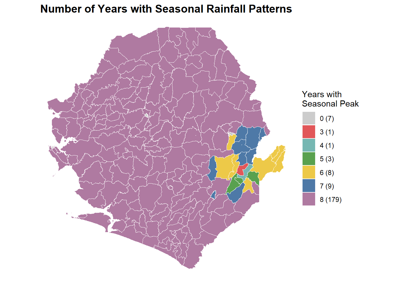
Step 9: Map years with seasonal peaks
This step creates a map showing how many years each location exhibited seasonal rainfall patterns. This visualization is useful for understanding the strength and consistency of seasonal signals across different areas. Locations that were seasonal in many years have strong, reliable patterns suitable for intervention planning, while locations with fewer seasonal years may have more variable rainfall patterns. The code prepares the data for mapping, defines a color scheme where different numbers of seasonal years receive different colors, and creates a map with a legend showing how many locations fall into each category.
Code
# Prepare data for mapping
merged$category <- as.character(merged$SeasonalYears)
merged$category[is.na(merged$category)] <- "0"

# Define color palette
category_colors <- c(
  "0" = "gray80",   # No seasonal years
  "1" = "#4E79A7",  "2" = "#F28E2B", "3" = "#E15759",
  "4" = "#76B7B2",  "5" = "#59A14F", "6" = "#EDC948",
  "7" = "#4E79A7",  "8" = "#AF7AA1"
)

# Convert to factor with proper ordering
merged$category <- factor(merged$category, levels = as.character(0:8))

# Count locations in each category
cat_counts <- table(merged$category)
cat_counts <- cat_counts[cat_counts > 0]

# Create legend labels with counts
legend_labels <- paste0(names(cat_counts), " (", cat_counts, ")")
names(legend_labels) <- names(cat_counts)

# Filter colors to categories that exist
category_colors_filtered <- category_colors[names(category_colors) %in% names(cat_counts)]

# Create map
p <- ggplot(merged) +
  geom_sf(aes(fill = category), color = "white", size = 0.2) +
  scale_fill_manual(
    values = category_colors_filtered,
    labels = legend_labels,
    name = "Years with\nSeasonal Peak"
  ) +
  theme_void() +
  theme(
    legend.position = "right",
    plot.title = element_text(hjust = 0.5, size = 14, face = "bold")
  ) +
  labs(title = "Number of Years with Seasonal Rainfall Patterns")

print(p)
Output
To adapt the code:
Lines 11-15: Modify color palette if desired
Line 43: Change map title as needed
The map above shows how many years each chiefdom in Sierra Leone experienced seasonal rainfall patterns based on the 60 percent threshold. Areas in deep purple had seasonal peaks in all eight years, indicating strong and consistent seasonality suitable for SMC implementation. Lighter colors such as blue, yellow, and red represent locations with fewer seasonal years, showing more variable rainfall patterns. The legend summarizes how many chiefdoms fall into each category, helping identify areas with stable versus inconsistent seasonality for program planning.
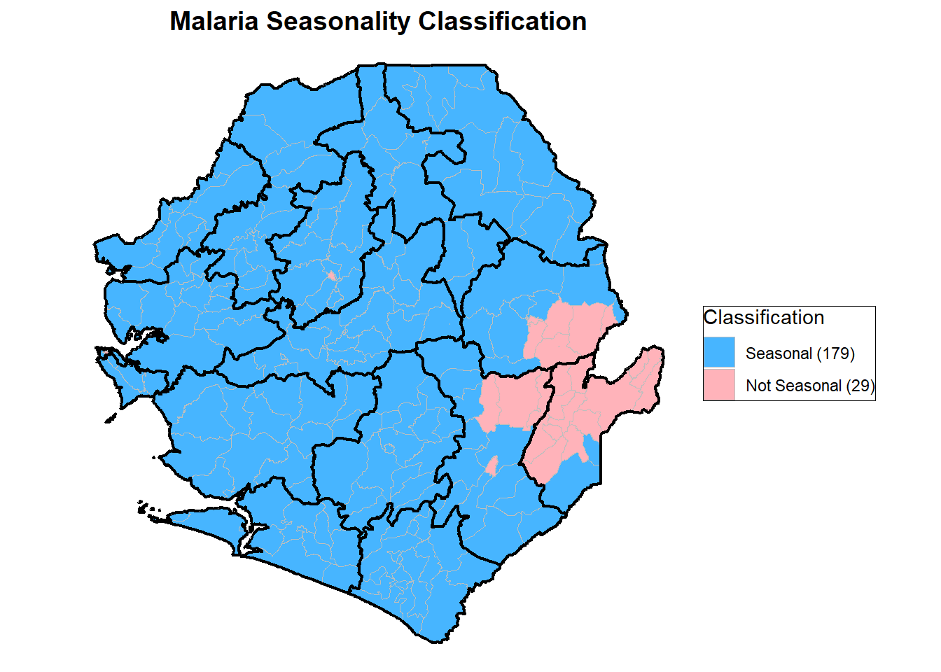
Step 10: Map final seasonality classification
This step generates the final seasonality classification map, distinguishing areas as Seasonal or Not Seasonal based on the consistency of rainfall patterns. The process involves preparing the dataset, defining a two-color scheme (blue for Seasonal and light pink for Not Seasonal), and creating district boundaries by dissolving chiefdom polygons for clearer geographic reference. The seasonality variable is converted to an ordered factor for proper legend arrangement, and the number of locations in each category is counted to label the legend (e.g., “Seasonal (89)”).
Code
# Handle missing values
merged$Seasonality[is.na(merged$Seasonality)] <- "No data"

# Define colors
colors <- c(
  "Seasonal" = "#47B5FF",
  "Not Seasonal" = "#FFB3BA",
  "No data" = "white"
)

# Create district boundaries for overlay
boundaries <- merged |>
  dplyr::group_by(FIRST_DNAM) |>
  dplyr::summarise(geometry = sf::st_union(geometry))

# Convert to factor
merged$Seasonality <- factor(
  merged$Seasonality,
  levels = c("Seasonal", "Not Seasonal", "No data")
)

# Count categories
cat_counts <- table(merged$Seasonality)
cat_counts <- cat_counts[cat_counts > 0]

# Create legend labels with counts
legend_labels <- paste0(names(cat_counts), " (", cat_counts, ")")
names(legend_labels) <- names(cat_counts)

# Filter colors
colors_filtered <- colors[names(colors) %in% names(cat_counts)]

# Create final map
p <- ggplot() +
  geom_sf(data = merged, aes(fill = Seasonality),
          color = "gray", linewidth = 0.3) +
  geom_sf(data = boundaries, fill = NA,
          color = "black", linewidth = 0.8) +
  scale_fill_manual(
    values = colors_filtered,
    labels = legend_labels,
    name = "Classification"
  ) +
  labs(title = "Malaria Seasonality Classification") +
  theme_void() +
  theme(
    plot.title = element_text(hjust = 0.5, size = 14, face = "bold"),
    legend.position = "right",
    legend.background = element_rect(fill = "white", color = "black")
  )

print(p)
Output
To adapt the code:
Lines 6-9: Modify colors for seasonal and non-seasonal categories to match your organization’s style
Lines 13-15: Change grouping variable (
FIRST_DNAM) if you want boundaries at a different admin levelLine 44: Update map title as needed
The map above shows how chiefdoms in Sierra Leone were classified based on rainfall consistency. Areas in blue are Seasonal, meaning they consistently had at least 60 percent of annual rainfall within a four month period across all analyzed years. These 179 chiefdoms have stable and predictable rainfall patterns that make them suitable for time bound malaria interventions such as Seasonal Malaria Chemoprevention. Areas in pink are Not Seasonal, representing 29 chiefdoms with irregular or inconsistent rainfall patterns. Most parts of Sierra Leone are classified as Seasonal, while a few areas in the east and south show variability that may require further review or different intervention timing.
Summary
This section explains how to identify and classify malaria seasonality using rainfall data based on the WHO four-month rule. It applies a rolling window approach to detect periods when at least 60 percent of annual rainfall occurs within any four consecutive months and determines whether this pattern is consistent across multiple years. The analysis produces yearly and location-level classifications of “Seasonal” and “Not Seasonal,” supported by clear maps and summaries. These outputs help programs align intervention timing, such as SMC and IRS campaigns, with predictable rainfall and transmission cycles.
Full Code
Find the full code for seasonality stratification below.
# ============================
# Step 1: Import packages and data
# ============================
if (!requireNamespace("pacman", quietly = TRUE)) install.packages("pacman")

pacman::p_load(
  readxl, dplyr, openxlsx, lubridate, ggplot2, readr, stringr,
  here, tidyr, gridExtra, knitr, writexl, sf
)

# File path
file_path <- here::here("english/data_r/modeled", "chirps_data_2015_2023_lastest.xls")

# Load your data
data <- readxl::read_excel(file_path)


# ============================
# Step 2: Configure analysis parameters
# ============================
year_column <- "Year"
month_column <- "Month"
value_column <- "mean_rain"
admin_columns <- c("FIRST_DNAM", "FIRST_CHIE")

analysis_start_year <- 2015
analysis_start_month <- 1
seasonality_threshold <- 60

#detailed_output <- "detailed_seasonality_results.xlsx"
#yearly_output <- "yearly_analysis_summary.xlsx"
#location_output <- "location_seasonality_summary.xlsx"


# ============================
# Step 3: Prepare data for analysis
# ============================
required_cols <- c(year_column, month_column, value_column, admin_columns)
missing_cols <- required_cols[!required_cols %in% colnames(data)]
if (length(missing_cols) > 0) {
  stop(paste("Missing columns:", paste(missing_cols, collapse = ", ")))
}

filtered_data <- data |>
  dplyr::filter(
    !is.na(!!sym(year_column)) &
    !is.na(!!sym(month_column)) &
    !!sym(year_column) >= analysis_start_year
  ) |>
  dplyr::mutate(Month = as.numeric(!!sym(month_column)))

if (length(admin_columns) == 1) {
  filtered_data$admin_group <- filtered_data[[admin_columns[1]]]
} else {
  filtered_data <- filtered_data |>
    dplyr::mutate(
      admin_group = paste(!!!syms(admin_columns), sep = " | ")
    )
}

available_years <- sort(unique(filtered_data[[year_column]]))
data_span_years <- length(available_years)

if (data_span_years < 6) {
  stop(paste(
    "Insufficient data: Analysis requires at least 6 years of data, but only",
    data_span_years, "years found."
  ))
}

num_complete_years <- data_span_years - 1
total_num_blocks <- num_complete_years * 12


# ============================
# Step 4: Generate rolling time blocks
# ============================
month_names <- c("Jan", "Feb", "Mar", "Apr", "May", "Jun",
                 "Jul", "Aug", "Sep", "Oct", "Nov", "Dec")

blocks <- data.frame()
current_year <- analysis_start_year
current_month <- analysis_start_month

for (i in 1:total_num_blocks) {
  # 4-month period
  start_4m_year <- current_year
  start_4m_month <- current_month
  end_4m_year <- current_year
  end_4m_month <- current_month + 3

  if (end_4m_month > 12) {
    end_4m_year <- end_4m_year + 1
    end_4m_month <- end_4m_month - 12
  }

  # 12-month period
  start_12m_year <- current_year
  start_12m_month <- current_month
  end_12m_year <- current_year
  end_12m_month <- current_month + 11

  if (end_12m_month > 12) {
    end_12m_year <- end_12m_year + 1
    end_12m_month <- end_12m_month - 12
  }

  # Create date range label
  date_range <- paste0(
    month_names[start_4m_month], " ", start_4m_year, "-",
    month_names[end_4m_month], " ", end_4m_year
  )

  # Store block information
  blocks <- rbind(blocks, data.frame(
    block_number = i,
    start_4m_year = start_4m_year,
    start_4m_month = start_4m_month,
    end_4m_year = end_4m_year,
    end_4m_month = end_4m_month,
    start_12m_year = start_12m_year,
    start_12m_month = start_12m_month,
    end_12m_year = end_12m_year,
    end_12m_month = end_12m_month,
    date_range = date_range
  ))

  # Move to next month
  current_month <- current_month + 1
  if (current_month > 12) {
    current_month <- 1
    current_year <- current_year + 1
  }
}


# ============================
# Step 5: Calculate seasonality for each block
# ============================
detailed_results <- data.frame()
admin_groups <- unique(filtered_data$admin_group)

for (admin_unit in admin_groups) {
  unit_data <- filtered_data |> dplyr::filter(admin_group == admin_unit)

  for (i in 1:nrow(blocks)) {
    block <- blocks[i, ]
    unit_data_ym <- unit_data[[year_column]] * 12 + unit_data$Month

    # 4-month window
    start_4m_ym <- block$start_4m_year * 12 + block$start_4m_month
    end_4m_ym <- block$end_4m_year * 12 + block$end_4m_month
    data_4m <- unit_data |> dplyr::filter(unit_data_ym >= start_4m_ym & unit_data_ym <= end_4m_ym)
    total_4m <- sum(data_4m[[value_column]], na.rm = TRUE)

    # 12-month window
    start_12m_ym <- block$start_12m_year * 12 + block$start_12m_month
    end_12m_ym <- block$end_12m_year * 12 + block$end_12m_month
    data_12m <- unit_data |> dplyr::filter(unit_data_ym >= start_12m_ym & unit_data_ym <= end_12m_ym)
    total_12m <- sum(data_12m[[value_column]], na.rm = TRUE)

    # Percentage & flag
    percent_seasonality <- ifelse(total_12m > 0, (total_4m / total_12m) * 100, 0)
    is_seasonal <- as.numeric(percent_seasonality >= seasonality_threshold)

    # Build result row
    result_row <- data.frame(
      Block = i, DateRange = block$date_range,
      Total_4M = total_4m, Total_12M = total_12m,
      Percent_Seasonality = round(percent_seasonality, 2),
      Seasonal = is_seasonal,
      stringsAsFactors = FALSE
    )

    if (length(admin_columns) > 1) {
      admin_parts <- strsplit(admin_unit, " \\| ")[[1]]
      for (j in seq_along(admin_columns)) {
        result_row[[admin_columns[j]]] <- ifelse(j <= length(admin_parts), admin_parts[j], NA)
      }
    } else {
      result_row[[admin_columns[1]]] <- admin_unit
    }

    detailed_results <- rbind(detailed_results, result_row)
  }
}

# Preview results
knitr::kable(head(detailed_results), caption = "Preview of Detailed Block Results")


# ============================
# Step 6: Generate yearly summary
# ============================
detailed_results$StartYear <- sapply(detailed_results$DateRange, function(x) {
  parts <- strsplit(x, "-")[[1]]
  first_part <- trimws(parts[1])
  as.numeric(substr(first_part, nchar(first_part) - 3, nchar(first_part)))
})

yearly_summary <- detailed_results |>
  dplyr::group_by(dplyr::across(dplyr::all_of(admin_columns)), StartYear) |>
  dplyr::summarise(
    Year = dplyr::first(StartYear),
    SeasonalCount = sum(Seasonal, na.rm = TRUE),
    total_blocks_in_year = 12,
    at_least_one_seasonal_block = as.numeric(SeasonalCount > 0),
    .groups = 'drop'
  ) |>
  dplyr::mutate(
    year_period = paste0(
      "(Jan ", Year, "-Apr ", Year, ", Dec ", Year, "-Mar ", Year + 1, ")"
    )
  ) |>
  dplyr::select(
    Year, dplyr::all_of(admin_columns),
    year_period, total_blocks_in_year, at_least_one_seasonal_block
  ) |>
  dplyr::arrange(Year, dplyr::across(dplyr::all_of(admin_columns)))

# Preview summary
knitr::kable(tail(yearly_summary, 10), caption = "Yearly Seasonality Summary (Last 10 rows)")


# ============================
# Step 7: Location-level seasonality classification
# ============================
location_summary <- yearly_summary |>
  dplyr::group_by(dplyr::across(dplyr::all_of(admin_columns))) |>
  dplyr::summarise(
    SeasonalYears = sum(at_least_one_seasonal_block, na.rm = TRUE),
    TotalYears = dplyr::n(),
    .groups = 'drop'
  ) |>
  dplyr::mutate(
    Seasonality = ifelse(SeasonalYears == TotalYears, "Seasonal", "Not Seasonal")
  ) |>
  dplyr::arrange(dplyr::across(dplyr::all_of(admin_columns)))

# Preview classification
knitr::kable(head(location_summary, 10), caption = "Location Seasonality Classification")


# ============================
# Step 8: Merge data for visualization
# ============================
file_path <- here::here("english/data_r/shapefiles", "Chiefdom2021.shp")
file_path_2 <- here::here("english/library/stratification/other", "final_SMC_eligibility.xlsx")

spatial_data <- sf::st_read(file_path)
category_data <- readxl::read_excel(file_path_2)

merged <- spatial_data |>
  dplyr::left_join(category_data, by = c("FIRST_DNAM", "FIRST_CHIE"))


# ============================
# Step 9: Map for years of seasonal peak
# ============================
merged$category <- as.character(merged$SeasonalYears)
merged$category[is.na(merged$category)] <- "0"

category_colors <- c(
  "0" = "gray80",
  "1" = "#4E79A7", "2" = "#F28E2B", "3" = "#E15759",
  "4" = "#76B7B2", "5" = "#59A14F", "6" = "#EDC948",
  "7" = "#4E79A7", "8" = "#AF7AA1"
)

merged$category <- factor(merged$category, levels = as.character(0:8))

cat_counts <- table(merged$category)
cat_counts <- cat_counts[cat_counts > 0]

legend_labels <- paste0(names(cat_counts), " (", cat_counts, ")")
names(legend_labels) <- names(cat_counts)

category_colors_filtered <- category_colors[names(category_colors) %in% names(cat_counts)]

p <- ggplot(merged) +
  geom_sf(aes(fill = category), color = "white", size = 0.2) +
  scale_fill_manual(values = category_colors_filtered, labels = legend_labels, name = "Category") +
  theme_minimal() + theme_void() +
  theme(
    legend.position = "right",
    plot.title = element_text(hjust = 0.5, size = 14, face = "bold"),
    panel.grid = element_blank()
  ) +
  labs(title = "Map by Category (0-8)")

print(p)

### Seasonality plot

# Replace NA with "No data" if needed
merged$Seasonality[base::is.na(merged$Seasonality)] <- "No data"

# Assign colors
colors <- c(
  "Seasonal" = "#47B5FF",      # Blue
  "Not Seasonal" = "#FFB3BA",  # Light pink
  "No data" = "white"
)

# Boundaries for FIRST_DNAM
boundaries <- merged |>
  dplyr::group_by(FIRST_DNAM) |>
  dplyr::summarise(geometry = sf::st_union(geometry))

# Convert to factor
merged$Seasonality <- base::factor(
  merged$Seasonality,
  levels = c("Seasonal", "Not Seasonal", "No data")
)

# Count categories (excluding zero counts)
cat_counts <- base::table(merged$Seasonality)
cat_counts <- cat_counts[cat_counts > 0]

# Create labels with counts
legend_labels <- base::paste0(base::names(cat_counts), " (", cat_counts, ")")
base::names(legend_labels) <- base::names(cat_counts)

# Filter colors to only include categories that exist
colors_filtered <- colors[base::names(colors) %in% base::names(cat_counts)]

# Plot
p <- ggplot2::ggplot() +
  ggplot2::geom_sf(data = merged, ggplot2::aes(fill = Seasonality),
                   color = "gray", linewidth = 0.3) +
  ggplot2::geom_sf(data = boundaries, fill = NA,
                   color = "black", linewidth = 0.8) +
  ggplot2::scale_fill_manual(
    values = colors_filtered,
    labels = legend_labels,
    name = "Seasonality"
  ) +
  ggplot2::labs(title = "Malaria Seasonality Classification") +
  ggplot2::theme_void() +
  ggplot2::theme(
    plot.title = ggplot2::element_text(hjust = 0.5, size = 14, face = "bold"),
    legend.position = "right",
    legend.background = ggplot2::element_rect(fill = "white", color = "black"),
    legend.key = ggplot2::element_rect(color = "black")
  )

# Display plot
base::print(p)