################################################################################
################ ~ ITN ownership, access, and usage full code ~ ################
################################################################################
### Step -----------------------------------------------------------------------
#### Step 1: Install or load required packages ---------------------------------
# install or load required packages
pacman::p_load(
  rdhs, # DHS API access and dataset management
  here, # safe relative file paths across machines/projects
  glue, # string interpolation for filenames, labels, etc.
  tidyverse, # includes dplyr, tidyr, readr, ggplot2 for data wrangling & viz
  labelled, # manage and preserve variable labels from DHS .dta files
  haven, # read Stata files and work with labelled data
  survey, # apply DHS weights and compute design-based statistics
  sf, # handle shapefiles and geospatial operations
  forcats, # factor manipulation and releveling
  ggplot2, # plotting
  viridis, # colorblind-friendly palettes for maps
  rio, # import/export to multiple file formats
  cowplot # for combining multiple plots
)

#' Check DHS Indicator List from API
#'
#' @param countryIds DHS country code(s), e.g., "EG"
#' @param indicatorIds Specific indicator ID(s)
#' @param surveyIds Survey ID(s)
#' @param surveyYear Exact year
#' @param surveyYearStart Start of year range
#' @param surveyYearEnd End of year range
#' @param surveyType DHS survey type (e.g., "DHS", "MIS")
#' @param surveyCharacteristicIds Filter by survey characteristic ID
#' @param tagIds Filter by tag ID
#' @param returnFields Fields to return
#'   (default: IndicatorId, Label, Definition)
#' @param perPage Max results per page (default = 500)
#' @param page Specific page to return (default = 1)
#' @param f Format (default = "json")
#'
#' @return A data.frame of indicators
#' @export
check_dhs_indicators <- function(
  countryIds = NULL,
  indicatorIds = NULL,
  surveyIds = NULL,
  surveyYear = NULL,
  surveyYearStart = NULL,
  surveyYearEnd = NULL,
  surveyType = NULL,
  surveyCharacteristicIds = NULL,
  tagIds = NULL,
  returnFields = c("IndicatorId", "Label", "Definition", "MeasurementType"),
  perPage = NULL,
  page = NULL,
  f = "json"
) {
  # Base URL
  base_url <- "https://api.dhsprogram.com/rest/dhs/indicators?"

  # Build query string
  params <- list(
    countryIds = countryIds,
    indicatorIds = indicatorIds,
    surveyIds = surveyIds,
    surveyYear = surveyYear,
    surveyYearStart = surveyYearStart,
    surveyYearEnd = surveyYearEnd,
    surveyType = surveyType,
    surveyCharacteristicIds = surveyCharacteristicIds,
    tagIds = tagIds,
    returnFields = paste(returnFields, collapse = ","),
    perPage = perPage,
    page = page,
    f = f
  )

  # Drop NULLs and encode
  query <- paste(
    purrr::compact(params) |>
      purrr::imap_chr(
        ~ paste0(.y, "=", URLencode(as.character(.x), reserved = TRUE))
      ),
    collapse = "&"
  )

  # Full URL
  full_url <- paste0(base_url, query)

  # Fetch with progress bar
  response <- httr::GET(full_url, httr::progress())
  jsonlite::fromJSON(httr::content(
    response,
    as = "text",
    encoding = "UTF-8"
  ))$Data
}

#' Query DHS API Directly via URL Parameters
#'
#' Builds and queries DHS API for indicator data using URL-based access
#' instead of rdhs package.
#'
#' @param countryIds Comma-separated DHS country code(s), e.g., "SL"
#' @param indicatorIds Comma-separated DHS indicator ID(s),
#'   e.g., "CM_ECMR_C_U5M"
#' @param surveyIds Optional comma-separated survey ID(s), e.g., "SL2016DHS"
#' @param surveyYear Optional exact survey year, e.g., "2016"
#' @param surveyYearStart Optional survey year range start
#' @param surveyYearEnd Optional survey year range end
#' @param breakdown One of: "national", "subnational", "background", "all"
#' @param f Format to return (default is "json")
#'
#' @return A data.frame containing the `Data` portion of the API response.
#' @export
download_dhs_indicators <- function(
  countryIds,
  indicatorIds,
  surveyIds = NULL,
  surveyYear = NULL,
  surveyYearStart = NULL,
  surveyYearEnd = NULL,
  breakdown = "subnational",
  f = "json"
) {
  # Base URL
  base_url <- "https://api.dhsprogram.com/rest/dhs/data?"

  # Assemble query string
  query <- paste0(
    "breakdown=",
    breakdown,
    "&indicatorIds=",
    indicatorIds,
    "&countryIds=",
    countryIds,
    if (!is.null(surveyIds)) paste0("&surveyIds=", surveyIds),
    if (!is.null(surveyYear)) paste0("&surveyYear=", surveyYear),
    if (!is.null(surveyYearStart)) paste0(
      "&surveyYearStart=", surveyYearStart
    ),
    if (!is.null(surveyYearEnd)) paste0("&surveyYearEnd=", surveyYearEnd),
    "&lang=en&f=",
    f
  )

  full_url <- paste0(base_url, query)

  cli::cli_alert_info("Downloading DHS data...")

  response <- httr::GET(full_url, httr::progress())

  if (httr::http_error(response)) {
    stop("API request failed: ", httr::status_code(response))
  }

  content_raw <- httr::content(response, as = "text", encoding = "UTF-8")
  data <- jsonlite::fromJSON(content_raw)$Data

  cli::cli_alert_success("Download complete: {nrow(data)} records retrieved.")
  return(data)
}
#### Step 2: Download the relevant indicators ----------------------------------
# Get ITN ownership data at subnational level
hh_own_dhs_ind <- download_dhs_indicators(
  countryIds = "SL",
  surveyYear = 2019,
  indicatorIds = "ML_NETP_H_ITN",
  breakdown = "subnational"
) |>
  dplyr::mutate(
    dhs_indicator_id = "ML_NETP_H_ITN",
    indicator = "Household ITN Ownership"
  ) |>
  dplyr::select(
    dhs_indicator_id, indicator,
    adm2_code = RegionId, pct = Value
  )

# Get ITN access data at subnational level
indiv_access_dhs_ind <- download_dhs_indicators(
  countryIds = "SL",
  surveyYear = 2019,
  indicatorIds = "ML_ITNA_P_ACC",
  breakdown = "subnational"
) |>
  dplyr::mutate(
    dhs_indicator_id = "ML_ITNA_P_ACC",
    indicator = "Individual ITN Access in all Population"
  ) |>
  dplyr::select(
    dhs_indicator_id, indicator,
    adm2_code = RegionId, pct = Value
  )
#### Step 3: Join indicators with shapefile ------------------------------------
# Get the DHS adm2 shapefile
sle_dhs_shp2 <- sf::read_sf(
  here::here(
    "01_foundational/1a_administrative_boundaries",
    "1ai_adm2",
    "sdr_subnational_boundaries_adm2.shp"
  )
) |>
  dplyr::select(
    adm1 = OTHREGNA,
    adm2 = DHSREGEN,
    adm2_code = REG_ID
  ) |>
  # Make adm1 and adm2 to upper case
  dplyr::mutate(
    adm1 = toupper(adm1),
    adm2 = toupper(adm2)
  )

# Bind indicators into one dataset
dhs_api_indi <- dplyr::bind_rows(hh_own_dhs_ind, indiv_access_dhs_ind) |>
  # Join adm2 DHS shapefile to data only keeping adm2 indicators
  dplyr::inner_join(sle_dhs_shp2, by = "adm2_code") |>
  # select only relevant columns
  dplyr::select(dhs_indicator_id, indicator, adm1, adm2, pct, geometry) |>
  sf::st_as_sf()

# check indicators
sf::st_drop_geometry(dhs_api_indi)
#### Step 4: Visualize subnational indicator data ------------------------------
# categorise the props
dhs_api_indi_final <- dhs_api_indi |>
  dplyr::mutate(
    prop_cat = cut(
      pct,
      breaks = c(0, 10, 20, 30, 40, 50, 60, 70, 80, 90, 100),
      labels = c(
        "<10",
        "10 to <20",
        "20 to <30",
        "30 to <40",
        "40 to <50",
        "50 to <60",
        "60 to <70",
        "70 to <80",
        "80 to <90",
        "90 to 100"
      ),
      include.lowest = TRUE,
      right = FALSE
    )
  )

# visualize the results
map1 <- dhs_api_indi_final |>
  dplyr::filter(indicator == "Household ITN Ownership") |>
  ggplot2::ggplot() +
  ggplot2::geom_sf(
    ggplot2::aes(fill = prop_cat),
    color = "black",
    size = 2,
    show.legend = TRUE
  ) +
  ggplot2::scale_fill_manual(
    name = "% Category",
    values = c(
      "<10" = "#9E0142",
      "10 to <20" = "#D53E4F",
      "20 to <30" = "#F46D43",
      "30 to <40" = "#FDAE61",
      "40 to <50" = "#FEE08B",
      "50 to <60" = "#E6F598",
      "60 to <70" = "#ABDDA4",
      "70 to <80" = "#66C2A5",
      "80 to <90" = "#3288BD",
      "90 to 100" = "#5E4FA2"
    ),
    drop = FALSE
  ) +
  ggplot2::labs(
    title = "Household ITN Ownership"
  ) +
  ggplot2::theme_void() +
  ggplot2::theme(
    legend.title = ggplot2::element_text(face = "bold"),
    legend.text = ggplot2::element_text(size = 10)
  )

# visualize the results
map2 <- dhs_api_indi_final |>
  dplyr::filter(indicator == "Individual ITN Access in All Population") |>
  ggplot2::ggplot() +
  ggplot2::geom_sf(
    ggplot2::aes(fill = prop_cat),
    color = "black",
    size = 2,
    show.legend = TRUE
  ) +
  ggplot2::scale_fill_manual(
    name = "% Category",
    values = c(
      "<10" = "#9E0142",
      "10 to <20" = "#D53E4F",
      "20 to <30" = "#F46D43",
      "30 to <40" = "#FDAE61",
      "40 to <50" = "#FEE08B",
      "50 to <60" = "#E6F598",
      "60 to <70" = "#ABDDA4",
      "70 to <80" = "#66C2A5",
      "80 to <90" = "#3288BD",
      "90 to 100" = "#5E4FA2"
    ),
    drop = FALSE
  ) +
  ggplot2::labs(
    title = "Individual ITN Access in all Population"
  ) +
  ggplot2::theme_void() +
  ggplot2::theme(
    legend.title = ggplot2::element_text(face = "bold"),
    legend.text = ggplot2::element_text(size = 10)
  )

# ensure legends are consistent for cowplot
common_legend <- cowplot::get_legend(
  map1
)

# remove legends from individual plots
plots_no_legend <- list(
  map1 +
    ggplot2::labs(subtitle = NULL, caption = NULL) +
    ggplot2::theme(legend.position = "none"),
  map2 +
    ggplot2::labs(subtitle = NULL, caption = NULL) +
    ggplot2::theme(legend.position = "none")
)

# combine maps in a grid (2 rows x 3 columns)
map_grid <- cowplot::plot_grid(
  plotlist = plots_no_legend,
  ncol = 2,
  align = "hv"
)

# add shared legend at the bottom
final_plot <- cowplot::plot_grid(
  map_grid,
  common_legend,
  nrow = 1,
  rel_widths = c(1, 0.2)
)

# print the final combined plot
final_plot
#### Step 2: Extract DHS data --------------------------------------------------
# import the HR (Household) data
sle_dhs_hr <- readRDS(
  here::here("1.6_health_systems/1.6a_dhs/raw/SLHR7AFL.rds")
)

# import the PR (Person) data
sle_dhs_pr <- readRDS(
  here::here("1.6_health_systems/1.6a_dhs/raw/SLPR7AFL.rds")
)
# select variables
sle_dhs_hr_final <- sle_dhs_hr |>
  dplyr::mutate(
    dhs_clust_num = hv001,
    hh_size = hv013,
    # calculate number of ITNs in household
    num_of_itns = sle_dhs_hr |>
      dplyr::select(dplyr::starts_with("hml10_")) |>
      rowSums(na.rm = TRUE),
    # prepare admin columns
    adm1 = haven::as_factor(hv024) |>
        toupper(),
    adm2 = haven::as_factor(shdist) |>
        toupper()
  ) |>
  dplyr::mutate(
    # calculate household-level ITN indicators
    hh_has_itn = as.integer(num_of_itns > 0),
    numerator = hh_size / num_of_itns,
    ratio_hh_2 = as.integer(numerator <= 2),
    potential_users = num_of_itns * 2,
    hh_sufficient_nets = as.integer((num_of_itns * 2) >= hh_size),
    survey_weight = hv005 / 1000000
  ) |>
  # select variables
  dplyr::select(
    hhid,
    dhs_clust_num,
    cluster_id = hv021,
    stratum_id = hv022,
    survey_weight,
    adm1,
    adm2,
    hh_size,
    num_of_itns,
    hh_has_itn,
    ratio_hh_2,
    potential_users,
    hh_sufficient_nets
  )


# label HR final dataset
sle_dhs_hr_final <- sle_dhs_hr_final |>
  labelled::set_variable_labels(
    hhid = "Household ID",
    dhs_clust_num = "DHS Cluster Number",
    cluster_id = "DHS Cluster ID",
    stratum_id = "DHS Stratum ID",
    survey_weight = "DHS Survey Weights",
    adm1 = "Admin Level 1",
    adm2 = "Admin Level 2",
    hh_size = "Household Size",
    num_of_itns = "Total ITNs in Household",
    hh_has_itn = "Owns ≥1 ITN",
    potential_users = "Potential ITN Users (2×ITNs)",
    hh_sufficient_nets = "Has Sufficient ITNs (≤2 Persons per ITN)",
  )
# merge with individual data and coordinate data
sle_pr_hr <- sle_dhs_hr_final |>
  dplyr::select(
    dhs_clust_num, hhid, hh_size,
    adm1, adm2, num_of_itns, hh_has_itn,
    ratio_hh_2, potential_users,
    hh_sufficient_nets) |>
  dplyr::right_join(sle_dhs_pr, by = "hhid")

# calculate individual-level indicators
sle_dhs_pr_hr_final <- sle_pr_hr |>
  dplyr::mutate(
    cluster_id = hv021,
    stratum_id = hv022,
    survey_weight = hv005 / 1000000,
    # sociodemographic factors
    age = hv105,
    age_group = cut(
      age,
      breaks = c(0, 5, 15, 30, 50, Inf),
      labels = c("0–4", "5–14", "15–29", "30–49", "50+"),
      right = FALSE
    ),
    sex = factor(
      hv104,
      levels = c(1, 2),
      labels = c("Male", "Female")
    ),
    is_pregnant_woman = factor(
      as.integer(hml18 == 1),
      levels = c(0, 1),
      labels = c("Not pregnant", "Pregnant")
    ),
    urban = dplyr::if_else(hv025 == 1, "urban", "rural"),
    wealth = dplyr::case_when(
      hv270 == 1 ~ "lowest",
      hv270 == 2 ~ "second",
      hv270 == 3 ~ "middle",
      hv270 == 4 ~ "fourth",
      hv270 == 5 ~ "highest"
    ),
    edu = dplyr::case_when(
      hv106 == 0 ~ "none",
      hv106 == 1 ~ "primary",
      hv106 %in% c(2, 3) ~ "high",
      hv106 == 8 ~ "unknown"
    ),
    potential_users = num_of_itns * 2,
    defacto_pop = hv013,
    used_itn_if_access = pmin(potential_users, defacto_pop),
    itn_access_ratio = used_itn_if_access / defacto_pop,
    itn_used = dplyr::if_else(hml12 %in% c(1, 2), 1L, 0L)
  ) |>
  # arrange individuals within each hh by ITN use (used first)
  dplyr::arrange(hhid, dplyr::desc(itn_used)) |>
  dplyr::group_by(hhid) |>
  dplyr::mutate(
    # assign person rank in household
    person_index = dplyr::row_number(),
    # assign individual access based on adjusted potential users
    net_access = dplyr::if_else(
      person_index <= used_itn_if_access, 1L, 0L),
    # used itn if individual had access
    used_itn_if_access = dplyr::if_else(
      net_access == 1L & itn_used == 1L, 1L, 0L)
  ) |>
  dplyr::ungroup() |>
  # select relevant vars
  dplyr::select(
    hhid, hvidx, hh_size, survey_weight, survey_weight,
    cluster_id, stratum_id, adm1, adm2, urban, sex, age,
    age_group, is_pregnant_woman, hh_has_itn, num_of_itns,
    hh_sufficient_nets, potential_users, itn_access_ratio,
    net_access, itn_used, used_itn_if_access,
    used_itn_if_access
  )

# label PR-HR final dataset
sle_dhs_pr_hr_final <-  sle_dhs_pr_hr_final |>
  labelled::set_variable_labels(
    hhid                           = "Household ID",
    hh_size                        = "Number of De Facto Household Members",
    survey_weight                  = "DHS Survey Weights",
    cluster_id                     = "DHS Cluster ID",
    stratum_id                     = "DHS Stratum ID",
    adm1                           = "Admin Level 1",
    adm2                           = "Admin Level 2",
    urban                          = "Urban/Rural Residence",
    sex                            = "Sex of Individual",
    age                            = "Age of Individual (Years)",
    age_group                      = "Age of Individual (Years, Categorised)",
    is_pregnant_woman              = "Individual is a Pregnant Woman",
    hh_has_itn                     = "Owns ≥1 ITN",
    num_of_itns                    = "Total ITNs in Household",
    hh_sufficient_nets             =
      "Has Sufficient ITNs (≤2 Persons per ITN)",
    potential_users                =
      "Potential ITN Users (2×Number of ITNs)",
    itn_access_ratio               =
      "Proportion of Household with Access to ITN",
    itn_used                       = "ITN Used Last Night (Binary)",
    used_itn_if_access             =
      "Standard Adjusted Potential Users (Capped)",
    used_itn_if_access             =
      "Used ITN Among Those with Standard Access"
  )
#### Step 3: Weighting ITN indicators ------------------------------------------
# define survey design object using DHS household weights
design_adm2_hr <- survey::svydesign(
  # defines the primary sampling unit (PSU):
  # typically the DHS cluster (hv021).
  ids = ~cluster_id,
  data = sle_dhs_hr_final,      # dhs dataset
  # specifies the stratification variable:
  # usually hv022 in DHS data.
  strata = ~stratum_id,
  # applies the household-level sampling weights,
  # derived as hv005/1,000,000.
  weights = ~survey_weight,
  # ensures that PSUs are nested within strata,
  # as per DHS sampling design.
  nest = TRUE
)

# calculate weighted proportion + 95% CI
pct_with_itn_by_adm2 <- survey::svyby(
  ~hh_has_itn,
  ~adm1 + adm2,
  design = design_adm2_hr,
  FUN = survey::svymean,
  vartype = c("ci"),  # add CI
  keep.names = F
) |>
  dplyr::mutate(
    pct = round(hh_has_itn * 100, 1),
    ci_low = round(ci_l * 100, 1),
    ci_upp = round(ci_u * 100, 1)
  ) |>
  dplyr::arrange(adm1) |>
  dplyr::select(adm1, adm2, pct, ci_low, ci_upp)

pct_with_itn_by_adm2
# define survey design object using DHS personal weights
design_adm2_pr <- survey::svydesign(
  ids = ~cluster_id,
  data = sle_dhs_pr_hr_final,
  strata = ~stratum_id,
  weights = ~survey_weight,
  nest = TRUE
)

# calculate weighted proportion + 95% CI
access_by_adm2 <- survey::svyby(
  ~itn_access_ratio,
  ~adm1 + adm2,
  design = design_adm2_pr,
  FUN = survey::svymean,
  vartype = c("ci"),
  keep.names = F
) |>
  dplyr::mutate(
    pct = round(itn_access_ratio * 100, 1),
    ci_low = round(ci_l * 100, 1),
    ci_upp = round(ci_u * 100, 1)
  ) |>
  dplyr::arrange(adm1) |>
  dplyr::select(adm1, adm2, pct, ci_low, ci_upp)

access_by_adm2
# calculate weighted proportion + 95% CI
itn_use_by_adm2 <- survey::svyby(
  ~itn_used,
  ~adm1 + adm2,
  design = design_adm2_pr,
  FUN = survey::svymean,
  vartype = c("ci"),
  keep.names = F
) |>
  dplyr::mutate(
    pct = round(itn_used * 100, 1),
    ci_low = round(ci_l * 100, 1),
    ci_upp = round(ci_u * 100, 1)
  ) |>
  dplyr::arrange(adm1) |>
  dplyr::select(adm1, adm2, pct, ci_low, ci_upp)

itn_use_by_adm2
# calculate usage among those with access by adm1
use_among_access_by_adm2 <- survey::svyby(
  ~used_itn_if_access,
  ~adm1 + adm2,
  design = design_adm2_pr,
  FUN = survey::svymean,
  vartype = c("ci"),
  keep.names = F
) |>
  dplyr::mutate(
    pct = round(used_itn_if_access * 100, 1),
    ci_low = round(ci_l * 100, 1),
    ci_upp = round(ci_u * 100, 1)
  ) |>
  dplyr::arrange(adm1) |>
  dplyr::select(adm1, adm2, pct, ci_low, ci_upp)

use_among_access_by_adm2
# calculate weighted proportion + 95% CI
pct_sufficient_itns_by_adm2 <- survey::svyby(
  ~hh_sufficient_nets,
  ~adm1 + adm2,
  design = design_adm2_hr,
  FUN = survey::svymean,
  vartype = c("ci"),
  keep.names = F
) |>
  dplyr::mutate(
    pct = round(hh_sufficient_nets * 100, 1),
    ci_low = round(ci_l * 100, 1),
    ci_upp = round(ci_u * 100, 1)
  ) |>
  dplyr::arrange(adm1) |>
  dplyr::select(adm1, adm2, pct, ci_low, ci_upp)

pct_sufficient_itns_by_adm2
#### Step 4: Stratified ITN indicators (e.g., by pregnancy) --------------------
# calculate weighted proportion + 95% CI by adm1 × age group
access_by_adm2_preg <- survey::svyby(
  ~itn_access_ratio,
  ~adm1 + adm2 + is_pregnant_woman,
  design = design_adm2_pr,
  FUN = survey::svymean,
  vartype = c("ci"),
  keep.names = FALSE
) |>
  dplyr::mutate(
    pct = round(itn_access_ratio * 100, 1),
    ci_low = round(ci_l * 100, 1),
    ci_upp = round(ci_u * 100, 1)
  ) |>
  dplyr::filter(is_pregnant_woman == "Pregnant") |>
  dplyr::arrange(adm1, adm2) |>
  dplyr::select(adm1, adm2, pct, ci_low, ci_upp)

access_by_adm2_preg
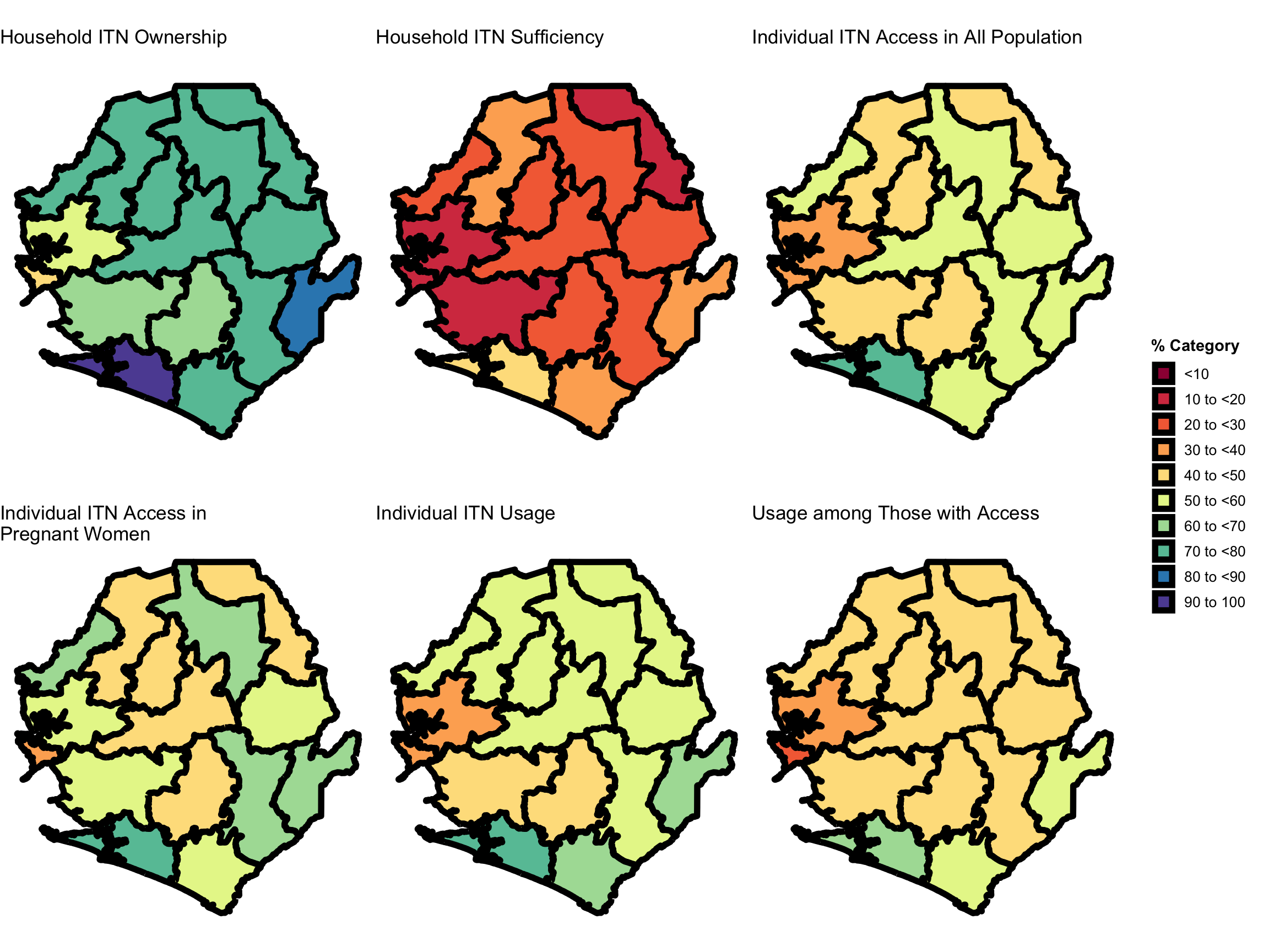
#### Step 5: Visualize household ITN ownership and usage -----------------------
joined_adm2_itn <- dplyr::bind_rows(
  pct_with_itn_by_adm2 |>
    dplyr::mutate(indicator = "Household ITN Ownership"),

  access_by_adm2 |>
    dplyr::mutate(indicator = "Individual ITN Access in All Population"),

  access_by_adm2_preg |>
    dplyr::mutate(indicator = "Individual ITN Access in Pregnant Women"),

  itn_use_by_adm2 |>
    dplyr::mutate(indicator = "Individual ITN Usage"),

  use_among_access_by_adm2 |>
    dplyr::mutate(indicator = "Usage among Those with Access"),

  pct_sufficient_itns_by_adm2 |>
    dplyr::mutate(indicator = "Household ITN Sufficiency")
) |>
  dplyr::relocate(indicator, .before = adm1)

head(joined_adm2_itn)
# join spatial data to itn final data
joined_adm2_itn_final <- joined_adm2_itn |>
  dplyr::left_join(
    sle_dhs_shp2,
    by = c("adm1", "adm2")
  ) |>
  sf::st_as_sf()

# define all possible categories
categories <- c(0, 10, 20, 30, 40, 50, 60, 70, 80, 90, 100)
labels <- c(
  "<10",
  "10 to <20",
  "20 to <30",
  "30 to <40",
  "40 to <50",
  "50 to <60",
  "60 to <70",
  "70 to <80",
  "80 to <90",
  "90 to 100"
)

# categorise pct
joined_adm2_itn_final <- joined_adm2_itn_final |>
  dplyr::mutate(
    pct_cat = cut(
      pct,
      breaks = categories,
      labels = labels,
      include.lowest = TRUE,
      right = FALSE
    ),
    pct_cat = factor(pct_cat, levels = labels)
  )

# set colours for plotting
category_colors <- c(
  "<10" = "#9E0142",
  "10 to <20" = "#D53E4F",
  "20 to <30" = "#F46D43",
  "30 to <40" = "#FDAE61",
  "40 to <50" = "#FEE08B",
  "50 to <60" = "#E6F598",
  "60 to <70" = "#ABDDA4",
  "70 to <80" = "#66C2A5",
  "80 to <90" = "#3288BD",
  "90 to 100" = "#5E4FA2"
)

# Visualize Household ITN Ownership by District
house_itn_own <- joined_adm2_itn_final |>
  dplyr::filter(indicator == "Household ITN Ownership") |>
  ggplot2::ggplot() +
  ggplot2::geom_sf(
    ggplot2::aes(fill = pct_cat),
    color = "black",
    size = 2,
    show.legend = TRUE
  ) +
  ggplot2::scale_fill_manual(
    name = "% Category",
    values = category_colors,
    drop = FALSE
  ) +
  ggplot2::labs(
    title = "Household ITN Ownership",
    subtitle = "Weighted estimates from the 2019 Sierra Leone DHS (HR dataset)",
    caption = "\nIndicator is shown as the percentage of the relevant households."
  ) +
  ggplot2::theme_void() +
  ggplot2::theme(
    legend.title = ggplot2::element_text(face = "bold"),
    legend.text = ggplot2::element_text(size = 10)
  )

# Visualize Individual ITN Access in all Population by District
indiv_itn_access <- joined_adm2_itn_final |>
  dplyr::filter(indicator == "Individual ITN Access in All Population") |>
  ggplot2::ggplot() +
  ggplot2::geom_sf(
    ggplot2::aes(fill = pct_cat),
    color = "black",
    size = 2,
    show.legend = TRUE
  ) +
  ggplot2::scale_fill_manual(
    name = "% Category",
    values = category_colors,
    drop = FALSE
  ) +
  ggplot2::labs(
    title = "Individual ITN Access in All Population",
    subtitle = "Weighted estimates from the 2019 Sierra Leone DHS (HR dataset)",
    caption = "\nIndicator is shown as the percentage of the relevant households."
  ) +
  ggplot2::theme_void() +
  ggplot2::theme(
    legend.title = ggplot2::element_text(face = "bold"),
    legend.text = ggplot2::element_text(size = 10)
  )

# Visualize Individual ITN Access in Pregnant Women by District
indiv_itn_access_preg <- joined_adm2_itn_final |>
  dplyr::filter(indicator == "Individual ITN Access in Pregnant Women") |>
  ggplot2::ggplot() +
  ggplot2::geom_sf(
    ggplot2::aes(fill = pct_cat),
    color = "black",
    size = 2,
    show.legend = TRUE
  ) +
  ggplot2::scale_fill_manual(
    name = "% Category",
    values = category_colors,
    drop = FALSE
  ) +
  ggplot2::labs(
    title = "Individual ITN Access in \nPregnant Women",
    subtitle = "Weighted estimates from the 2019 Sierra Leone DHS (HR dataset)",
    caption = "\nIndicator is shown as the percentage of the relevant households."
  ) +
  ggplot2::theme_void() +
  ggplot2::theme(
    legend.title = ggplot2::element_text(face = "bold"),
    legend.text = ggplot2::element_text(size = 10)
  )

# Visualize Individual ITN Usage by District
indiv_itn_usage <- joined_adm2_itn_final |>
  dplyr::filter(indicator == "Individual ITN Usage") |>
  ggplot2::ggplot() +
  ggplot2::geom_sf(
    ggplot2::aes(fill = pct_cat),
    color = "black",
    size = 2,
    show.legend = TRUE
  ) +
  ggplot2::scale_fill_manual(
    name = "% Category",
    values = category_colors,
    drop = FALSE
  ) +
  ggplot2::labs(
    title = "Individual ITN Usage",
    subtitle = "Weighted estimates from the 2019 Sierra Leone DHS (HR dataset)",
    caption = "\nIndicator is shown as the percentage of the relevant population"
  ) +
  ggplot2::theme_void() +
  ggplot2::theme(
    legend.title = ggplot2::element_text(face = "bold"),
    legend.text = ggplot2::element_text(size = 10)
  )

# Visualize Usage Among Those With Access by District

indiv_itn_usage_access <- joined_adm2_itn_final |>
  dplyr::filter(indicator == "Usage among Those with Access") |>
  ggplot2::ggplot() +
  ggplot2::geom_sf(
    ggplot2::aes(fill = pct_cat),
    color = "black",
    size = 2,
    show.legend = TRUE
  ) +
  ggplot2::scale_fill_manual(
    name = "% Category",
    values = category_colors,
    drop = FALSE
  ) +
  ggplot2::labs(
    title = "Usage among Those with Access",
    subtitle = "Weighted estimates from the 2019 Sierra Leone DHS (PR dataset)",
    caption = "\nIndicator is shown as the percentage of the relevant population"
  ) +
  ggplot2::theme_void() +
  ggplot2::theme(
    legend.title = ggplot2::element_text(face = "bold"),
    legend.text = ggplot2::element_text(size = 10)
  )

# Visualize Household ITN Sufficiency by District
house_suffic <- joined_adm2_itn_final |>
  dplyr::filter(indicator == "Household ITN Sufficiency") |>
  ggplot2::ggplot() +
  ggplot2::geom_sf(
    ggplot2::aes(fill = pct_cat),
    color = "black",
    size = 2,
    show.legend = TRUE
  ) +
  ggplot2::scale_fill_manual(
    name = "% Category",
    values = category_colors,
    drop = FALSE
  ) +
  ggplot2::labs(
    title = "Household ITN Sufficiency",
    subtitle = "Weighted estimates from the 2019 Sierra Leone DHS (HR dataset)",
    caption = "\nIndicator is shown as the percentage of the relevant households."
  ) +
  ggplot2::theme_void() +
  ggplot2::theme(
    legend.title = ggplot2::element_text(face = "bold"),
    legend.text = ggplot2::element_text(size = 10)
  )
# ensure legends are consistent for cowplot
common_legend <- cowplot::get_legend(
  house_itn_own
)

# remove legends from individual plots
plots_no_legend <- list(
  house_itn_own +
    ggplot2::labs(subtitle = NULL, caption = NULL) +
    ggplot2::theme(legend.position = "none"),
  house_suffic  +
    ggplot2::labs(subtitle = NULL, caption = NULL) +
    ggplot2::theme(legend.position = "none") ,
  indiv_itn_access +
    ggplot2::labs(subtitle = NULL, caption = NULL) +
    ggplot2::theme(legend.position = "none"),
  indiv_itn_access_preg +
    ggplot2::labs(subtitle = NULL, caption = NULL) +
    ggplot2::theme(legend.position = "none"),
  indiv_itn_usage +
    ggplot2::labs(subtitle = NULL, caption = NULL) +
    ggplot2::theme(legend.position = "none"),
  indiv_itn_usage_access +
    ggplot2::labs(subtitle = NULL, caption = NULL) +
    ggplot2::theme(legend.position = "none")
)

# combine maps in a grid (2 rows x 3 columns)
map_grid <- cowplot::plot_grid(
  plotlist = plots_no_legend,
  ncol = 3, align = "hv"
)

# add shared legend at the bottom
final_plot <- cowplot::plot_grid(
  map_grid,
  common_legend,
  nrow = 1,
  rel_widths = c(1, 0.125)
)

# print the final combined plot
final_plot
# Save Household ITN Ownership map
ggplot2::ggsave(
  plot = house_itn_own,
  filename = here::here("03_output/3a_figures/itn_ownership_adm2.png"),
  width = 12, height = 9, dpi = 300
)

# Save Individual ITN Access map
ggplot2::ggsave(
  plot = indiv_itn_access,
  filename = here::here("03_output/3a_figures/itn_access_adm2.png"),
  width = 12, height = 9, dpi = 300
)

# Save Individual ITN Access map for pregnant women
ggplot2::ggsave(
  plot = indiv_itn_access_preg,
  filename = here::here("03_output/3a_figures/itn_access_preg_adm2.png"),
  width = 12, height = 9, dpi = 300
)

# Save Individual ITN Usage map
ggplot2::ggsave(
  plot = indiv_itn_usage,
  filename = here::here("03_output/3a_figures/itn_usage_adm2.png"),
  width = 12, height = 9, dpi = 300
)

# Save Usage Among Those With Access map
ggplot2::ggsave(
  plot = indiv_itn_usage_access,
  filename = here::here(
    "03_output/3a_figures/itn_usage_among_with_access_adm2.png"
  ),
  width = 12, height = 9, dpi = 300
)

# Save Household ITN Sufficiency map
ggplot2::ggsave(
  plot = house_suffic,
  filename = here::here("03_output/3a_figures/itn_sufficiency_adm2.png"),
  width = 12, height = 9, dpi = 300
)

# Save all combined maps
ggplot2::ggsave(
  plot = final_plot,
  filename = here::here("03_output/3a_figures/itn_combined_maps_adm2.png"),
  width = 12, height = 9, dpi = 300
)
#### Step 6: Save processed ITN indicators -------------------------------------
# Define save directory
save_path <- here::here("1.6_health_systems/1.6a_dhs")

# Save HR dataset (household indicators)
rio::export(sle_dhs_hr_final,
            here::here(save_path, "processed", "sle_dhs_hr_final.csv"))

rio::export(sle_dhs_hr_final,
            here::here(save_path, "processed", "sle_dhs_hr_final.rds"))

# Save PR dataset (individual indicators)
rio::export(sle_dhs_pr_hr_final,
            here::here(save_path, "processed", "sle_dhs_pr_final.csv"))

rio::export(sle_dhs_pr_hr_final,
            here::here(save_path, "processed", "sle_dhs_pr_final.rds"))

# Save final joined ITN indicators with spatial data
rio::export(joined_adm2_itn_final |> sf::st_drop_geometry(),
            here::here(
              save_path,
              "processed",
              "final_weighted_adm2_itn_indicators.csv"
            ))

rio::export(joined_adm2_itn_final,
            here::here(
              save_path,
              "processed",
              "final_weighted_adm2_itn_indicators.rds"
            ))
-1.png)