Shapefile management and customization

Intermediate

Overview

In the SNT context, having an official, accurate, and up-to-date shapefile is important. These boundaries determine the scale at which we aggregate data, calculate indicators, apply targeting criteria, and visualize outputs. Misaligned or incomplete shapefiles can introduce serious errors, such as dropped areas, misclassified units, or misleading maps, which compromise both the validity of the analysis and its usefulness for decision-making.

Considerations for Managing and Customizing Shapefiles

Before a shapefile is used for any purpose, whether for joining data, visualizing maps, aggregating indicators, or running spatial analysis, it must be clean, valid, and properly structured. This section outlines key challenges and best practices in shapefile preparation that guide the reliability of all downstream steps in the SNT workflow. These steps form the data foundation on which reliable SNT analysis is built.

Valid and Complete Geometries

Shapefiles must be geometrically valid. Possible problems include:

spatial artifacts and overlaps from poor digitization
empty or zero-area polygons
multipart geometries or holes that affect containment logic.

Invalid geometries can silently break joins or misplace features. In SNT workflows, this may result in missing areas in coverage maps or unmatched clusters in analysis of survey data. It is always important to identify invalid geometries, flag them, and correct them where possible.

Ensuring Unique Polygons

Each unit in the shapefile should represent a single, distinct geographic area. Duplicate polygons, caused by digitization errors or mistakenly repeated records, can lead to incorrect joins, double-counting in aggregations, and confusion in mapping.

Why this matters: Duplicate features with the same name or ID can:

Distort summary statistics
Lead to incorrect matches when joining multiple shapefiles
Create misleading visualizations or maps

Possible issues to resolve:

Duplicate geometries (polygons or other geometry) with identical or repeated IDs
Multiple records representing the same unit

Example: If two features both have the name “Bumpe Ngao” and cover the same area, population estimates may be counted twice during zonal extraction or incidence calculations. One of the duplicates should be removed before using the shapefile.

We can use geospatial tools to detect and resolve duplicates, such as flagging repeated names or IDs, comparing geometries for equality, or dissolving features by administrative codes. We will demonstrate several examples in the Step-by-Step section below.

Coordinate Reference Systems (CRS)

For spatial joins to work correctly, both spatial data files must share the same CRS. A mismatch can cause points to fall outside their true polygons, even if coordinates are correct. Always confirm that both datasets use a common, appropriate CRS as mismatches can lead to misalignment and incorrect results. Typically WGS84 (EPSG:4326) is used. For more information on CRS, please visit Spatial data overview.

Aggregating or Reconstructing Admin Levels

Before starting any analysis, we should request all official shapefiles at the required unit of analysis and at all higher administrative levels. For example, if the chosen unit is adm2, we should also obtain the official adm1 shapefile. This is important for harmonizing data across levels and for producing SNT maps that include national and regional context and are easy to interpret.

In practice, we may find that the shapefile for the intended unit of analysis is missing or incomplete. For example, we might have data at adm2 but only a complete shapefile for adm3. In such cases, we can aggregate polygons from a more granular shapefile using a shared identifier to reconstruct the higher-level boundaries.

adm3 polygons can be grouped and dissolved by a common adm2 name or code to recreate adm2 boundaries. The same approach applies to adm1 boundaries.
We use this technique in SNT when reporting at broader levels (e.g., provinces or regions) or when visualizing national maps with consistent resolution, if dedicated shapefiles at the larger admin unit are not available.

Example: In Sierra Leone, if only adm3 boundaries are available, we can group adm3 units by their district name and merge their geometries. This reconstructs an adm2-level shapefile that matches the data and enables accurate mapping and aggregation.

This process ensures that the shapefile structure aligns with the level of the indicators and supports clean joins, visualizations, and reporting across administrative tiers.

Partial Aggregation for Flexible Resolution

In some cases, it may be beneficial to represent different parts of the country at different administrative levels within the same shapefile. For example, an SNT analysis might require adm3 detail for elimination areas, while the rest of the country can be visualized and analyzed at adm2.

This strategy is particularly useful when interventions or programmatic decisions require more granularity in some areas than others. It provides a practical way to balance detail and usability in maps and analysis while ensuring alignment with country-specific priorities and operational needs. This approach allows us to retain detailed boundaries in certain areas while using larger-unit boundaries elsewhere.

Handling mixed admin levels within a country

In some SNT exercises, countries choose to use different administrative levels in different regions, for instance, adm3 for urban areas and adm2 for rural zones. This reflects operational realities, data availability, or planning needs.

To support this hybrid setup, we can clip each shapefile to its relevant region and then merge them into a single boundary layer. With proper alignment of geometries and attributes, this structure allows for flexible, context-sensitive spatial analysis. The techniques needed to do this are covered on this page.

Tracking Boundary Changes

Administrative boundaries can shift over time, through redistricting, renaming, or reclassification. In SNT, it is important to detect these changes to ensure geographic consistency for time-series or trend analysis, and to make sure historical data is mapped and interpreted correctly.

While visualizing and comparing different versions of a shapefile by eye is a simple way to look for visible differences, it is also possible to detect changes more systematically and rigorously. One way to do this is by generating a geometry hash, a unique identifier based on a polygon’s coordinates. If a shape changes, its hash will change. If only the name or code changes but the geometry stays the same, the hash remains stable, making it easier to detect renames or confirm spatial continuity.

Example: If Kambia district’s geometry is unchanged but renamed across versions, its hash stays the same. If the shape is redrawn, the hash will differ, flagging it for review.

This approach supports version control, longitudinal consistency, and reproducible spatial workflows. Methods for computing and comparing hashes are covered later in this section.

Step-by-Step

In this section, we walk through the important steps to load, manage, troubleshoot, and customize shapefile data.

The example uses administrative boundary shapefiles from Sierra Leone, with focus on chiefdom (adm3) and district (adm2) levels. The principles can be applied to shapefiles from any country.

To skip the step-by-step explanation, jump to the full code at the end of this page.

Step 1: Install and load packages

First, install and/or load the necessary packages for handling spatial data, data manipulation, and visualization. These libraries provide the functions needed for working with spatial data.

The sf package is particularly important as it implements simple features standards for handling geographic vector data in R.

# install `pacman` if not already installed
if (!requireNamespace("pacman", quietly = TRUE)) {
  install.packages("pacman")
}

# load required packages using pacman
pacman::p_load(
  sf,         # handling shapefile data
  dplyr,      # data manipulation
  ggplot2,    # plotting
  here,       # file path management
  stringr,    # string manipulation (e.g., str_remove)
  cli,        # clean logging and CLI-style messages
  devtools    # for package management
)

# sntutils has a number of useful helper functions for
# data management and cleaning
if (!requireNamespace("sntutils", quietly = TRUE)) {
  devtools::install_github("ahadi-analytics/sntutils")
}

To adapt the code:

Do not modify anything in the code above.

Terminal installation required

Install packages in the terminal, if not already installed. For help installing packages, refer to the Getting Started page.

pip install pandas geopandas shapely matplotlib pyprojroot xxhash pyogrio pyarrow

Once packages are installed, load the relevant packages and define a few helper functions for plotting, geometry hashing, and geometry validation. These helpers keep the Python examples close to the R output style.

from pathlib import Path

import geopandas as gpd            # spatial vector data handling
import matplotlib.colors as mcolors
import matplotlib.patches as mpatches
import matplotlib.pyplot as plt    # plotting
import numpy as np                 # conditional logic and arrays
import pandas as pd                # data manipulation
import xxhash                      # fast stable hashing
from pyprojroot import here        # project-relative file paths
from shapely import make_valid
from shapely.geometry import GeometryCollection, MultiPolygon, Polygon
from shapely.ops import unary_union
from shapely.validation import explain_validity


def cli_info(message):
    """Print a simple message similar to cli::cli_alert_info()."""
    print(f"INFO: {message}")


def cli_header(message):
    """Print a simple section header similar to cli::cli_h1()/cli_h2()."""
    print(f"\n{message}")


def cli_success(message):
    """Print a success message similar to cli::cli_alert_success()."""
    print(f"SUCCESS: {message}")


def cli_warning(message):
    """Print a warning message similar to cli::cli_alert_warning()."""
    print(f"WARNING: {message}")


def cli_danger(message):
    """Print an error message similar to cli::cli_alert_danger()."""
    print(f"ERROR: {message}")


def sf_colors(n=10):
    """Match sf::sf.colors(..., categorical = TRUE) using matplotlib palettes."""
    palette_name = "Set2" if n <= 8 else "Set3"
    palette = [mcolors.to_hex(color) for color in plt.get_cmap(palette_name).colors]
    return [palette[i % len(palette)] for i in range(n)]


R_COLOR_MAP = {
    "grey10": "#1a1a1a",
    "gray10": "#1a1a1a",
    "grey30": "#4d4d4d",
    "gray30": "#4d4d4d",
    "grey90": "#e5e5e5",
    "gray90": "#e5e5e5",
}


def r_color(color):
    """Translate common R color names used here into matplotlib colors."""
    return R_COLOR_MAP.get(color, color)


def geometry_wkb(geom):
    """Return WKB bytes for exact-geometry duplicate checks."""
    if geom is None:
        return None
    return geom.wkb


def geometry_hash(geom, algo="xxhash32"):
    """Create a WKB-based geometry hash for duplicate and version checks."""
    if geom is None:
        return None
    payload = geom.wkb
    if algo == "xxhash32":
        return xxhash.xxh32(payload).hexdigest()
    if algo == "xxhash64":
        return xxhash.xxh64(payload).hexdigest()
    raise ValueError("Only xxhash32 and xxhash64 are implemented here.")


def polygonal_part(geom):
    """Keep polygonal output after make_valid() returns a GeometryCollection."""
    if geom is None or geom.is_empty:
        return geom
    if isinstance(geom, (Polygon, MultiPolygon)):
        return geom
    if isinstance(geom, GeometryCollection):
        pieces = [
            part for part in geom.geoms
            if isinstance(part, (Polygon, MultiPolygon))
        ]
        return unary_union(pieces) if pieces else geom
    return geom


def make_valid_polygonal(geom):
    """Python equivalent of sf::st_make_valid() for polygon layers."""
    return polygonal_part(make_valid(geom))


def as_geodataframe(data, crs=None):
    """Coerce a GeoDataFrame, GeoSeries, or geometry list to GeoDataFrame."""
    if isinstance(data, gpd.GeoDataFrame):
        return data
    if isinstance(data, gpd.GeoSeries):
        return gpd.GeoDataFrame(geometry=data, crs=data.crs)
    return gpd.GeoDataFrame(geometry=gpd.GeoSeries(data), crs=crs)


def plot_sf_like(
    data,
    ax=None,
    colors=None,
    border="grey10",
    linewidth=0.35,
    title=None,
    title_size=12,
):
    """Draw a map with styling close to base R sf plotting."""
    gdf = as_geodataframe(data)
    if ax is None:
        _, ax = plt.subplots()

    if colors is None:
        colors = sf_colors(len(gdf))
    elif isinstance(colors, str):
        colors = r_color(colors)
    else:
        colors = [r_color(colors[i % len(colors)]) for i in range(len(gdf))]

    gdf.plot(
        ax=ax,
        color=colors,
        edgecolor=r_color(border) if border else None,
        linewidth=linewidth,
    )
    ax.set_title(title or "", fontsize=title_size)
    ax.set_axis_off()
    ax.set_aspect("equal")
    return ax

To adapt the code:

Do not modify the import block unless the Python environment uses a different project-root helper or a package import fails.
Keep the helper functions in this first Python chunk. The plotting and geometry-hash sections below depend on them.

Step 2: Load and prepare shapefiles

Step 2.1: Load and examine data

Import both datasets and examine their structure to identify the appropriate join keys. This important step ensures understanding of the data before attempting to merge.

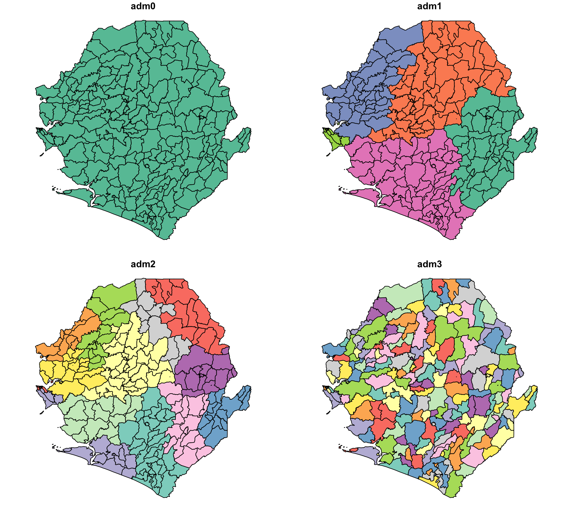
We begin by loading the Sierra Leone shapefile and selecting the relevant administrative levels for analysis. A new column for adm0 (country name) is added, and admin unit fields are renamed to standard adm1, adm2, and adm3 labels for consistency across the SNT workflow.

# set up spatial path
spat_path <- here::here(
  "01_data", "1.1_foundational", "1.1a_admin_boundaries"
)

# import shapefile
shp_adm3 <- sf::read_sf(
  here::here(spat_path, "raw", "Chiefdom2021.shp")
) |>
  dplyr::mutate(adm0 = "SIERRA LEONE") |>
  dplyr::select(
    # select relevant columns and rename to standard nomenclature
    adm0,
    adm1 = FIRST_REGI,
    adm2 = FIRST_DNAM,
    adm3 = FIRST_CHIE
  ) |>
  # ensure output remains a valid sf object for downstream usage
  sf::st_as_sf()

# check output by mapping
plot(shp_adm3)

Output

To adapt the code:

The code below shows how to modify the loading process when working with other spatial vector formats. All of these examples use sf::read_sf(), which supports multiple formats via GDAL.

GeoJSON: If the boundary file is in GeoJSON format, simply update the file extension

shp_adm3 <- sf::read_sf(
  here::here("folder", "boundary.geojson")  # path to geojson file
)

GeoPackage (.gpkg): For GeoPackage files, we must specify both the file and the layer name:

shp_adm3 <- sf::read_sf(
  here::here("folder", "boundary.gpkg"),    # path to gpkg file
  layer = "admin_boundaries"               # layer name inside gpkg
)

ℹ️ Use sf::st_layers("boundary.gpkg") to list all available layers in the file.

File Geodatabase (.gdb): For Geodatabase files, we must specify both the file and the layer name:

shp_adm3 <- sf::read_sf(
  "path/to/geodatabase.gdb",     # path to gdb
  layer = "admin_boundaries"    # layer name inside gdb
)

Once imported, the rest of the processing pipeline (mutate(), select(), st_set_crs(), etc.) remains the same.

Additional adaptations:

Lines 2–4: Change the here::here() path to match the folder structure.
Line 7: If working with a shapefile at a different admin unit level, change the variable name for the spatial object away from shp_adm3. For example, if working at adm2, shp_adm2 would be more appropriate.
Lines 13–16: Update the administrative column names (adm0, adm1, adm2, adm3) to reflect the dataset. For example, if the shapefile does not contain an adm3 level, remove the adm3 line.

# set up spatial path
spat_path = here("01_data/1.1_foundational/1.1a_admin_boundaries")

# import shapefile
shp_adm3 = (
    gpd.read_file(Path(spat_path) / "raw" / "Chiefdom2021.shp")
    .assign(adm0="SIERRA LEONE")
    .rename(columns={
        "FIRST_REGI": "adm1",
        "FIRST_DNAM": "adm2",
        "FIRST_CHIE": "adm3",
    })
    [["adm0", "adm1", "adm2", "adm3", "geometry"]]
)

# check output by mapping
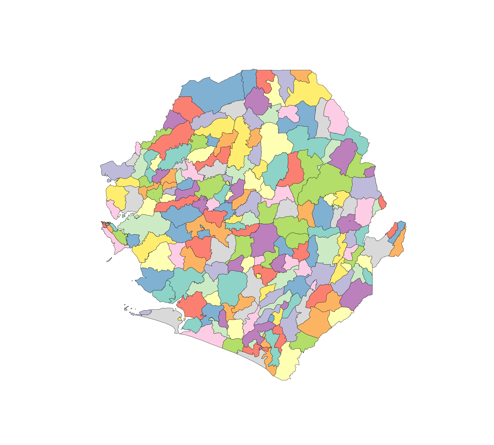
ax = plot_sf_like(shp_adm3, title="")
plt.show()

Output

GeoJSON: If the boundary file is in GeoJSON format, simply update the file extension

shp_adm3 = gpd.read_file(
    here("folder/boundary.geojson")  # path to geojson file
)

GeoPackage (.gpkg): For GeoPackage files, we must specify both the file and the layer name:

shp_adm3 = gpd.read_file(
    here("folder/boundary.gpkg"),    # path to gpkg file
    layer="admin_boundaries"         # layer name inside gpkg
)

Use gpd.list_layers("boundary.gpkg") to list all available layers in the file.

File Geodatabase (.gdb): For Geodatabase files, we must specify both the file and the layer name:

shp_adm3 = gpd.read_file(
    "path/to/geodatabase.gdb",       # path to gdb
    layer="admin_boundaries"         # layer name inside gdb
)

To adapt the code:

Line 2: Change the here() path to match the folder structure.
Line 5: If working with a shapefile at a different admin unit level, change the variable name away from shp_adm3, for example to shp_adm2.
Lines 10–14: Update the administrative column names (adm0, adm1, adm2, adm3) to reflect the dataset. If the shapefile does not contain an adm3 level, remove the adm3 line.
For GeoJSON, GeoPackage, and Geodatabase inputs, keep the downstream cleaning steps the same after gpd.read_file().

The R and Python maps look different because the default plot behaviour differs: R’s plot() on an sf object draws one panel per attribute, while Python’s GeoDataFrame.plot() renders a single map. The underlying data is identical.

Step 2.2: Check and transform CRS

Once loaded, it is important to ensure that the shapefile is in the appropriate coordinate reference system (CRS).

Below, we check the current CRS of the shapefile and, if needed, transform it to a consistent geographic reference system, to ensure all layers align correctly and will be compatible with other spatial datasets we might use.

The Sierra Leone shapefile is already in WGS84 (EPSG:4326), so normally we would not need to change the CRS. However, for demonstration purposes we provide an example of how to transform the CRS (to Equal Earth (EPSG:6933)).

cli::cli_h2("Check and assign original CRS for shp_adm3")
shp_adm3 <- sf::st_set_crs(shp_adm3, 4326)
cli::cli_alert_info("Original CRS: {sf::st_crs(shp_adm3)$input}")

# transform to new CRS (e.g., Equal Earth - EPSG:6933)
shp_adm3_diff_crs <- sf::st_transform(shp_adm3, 6933)

cli::cli_h2("Check CRS after transformation")
cli::cli_alert_info("New CRS: {sf::st_crs(shp_adm3_diff_crs)$input}")

Output

── Check and assign original CRS for shp_adm3 ──

ℹ Original CRS: EPSG:4326

── Check CRS after transformation ──

ℹ New CRS: EPSG:6933

To adapt the code:

Lines 1–2: Don’t change anything unless using a different variable for the shapefile object (e.g., shp_adm2) or a different CRS is needed.
Line 2: Use st_set_crs() only if the shapefile is missing a CRS but we are certain of what it should be. To reproject the geometry, always use st_transform().
Line 6: To use another projection, just update the EPSG code in st_transform(), for example to 4326 for the WGS84 CRS usually used in SNT, if the original shapefile had a different CRS.
If the shapefile was already in the correct CRS, lines 6 onwards can be removed.

cli_header("Check and assign original CRS for shp_adm3")
shp_adm3 = shp_adm3.set_crs(epsg=4326, allow_override=True)
cli_info(f"Original CRS: {shp_adm3.crs}")

# Transform to new CRS (e.g., Equal Earth - EPSG:6933)
shp_adm3_diff_crs = shp_adm3.to_crs(epsg=6933)

cli_header("Check CRS after transformation")
cli_info(f"New CRS: {shp_adm3_diff_crs.crs}")

Output


Check and assign original CRS for shp_adm3

INFO: Original CRS: EPSG:4326


Check CRS after transformation

INFO: New CRS: EPSG:6933

To adapt the code:

Lines 2–3: Replace shp_adm3 with the variable name for the relevant spatial object.
Line 3: Use .set_crs() only if the shapefile is missing a CRS and we are certain of what it should be. To reproject the geometry, always use .to_crs().
Line 7: To use another projection, update the EPSG code in .to_crs(epsg=...).
If the shapefile was already in the correct CRS, lines 6 onwards can be removed.

Step 3: Geometry validation

Step 3.1: Check and correct geometry validity

Invalid geometries, like overlaps, gaps, or broken shapes, can cause joins to fail or maps to misalign. These issues can go unnoticed but ultimately lead to missing areas or incorrect outputs. Before doing any joins, always check that the shapefile is valid.

# check geometry validity
shp_adm3_inv <- shp_adm3 |>
  dplyr::mutate(
    valid = sf::st_is_valid(geometry),
    invalid_reason = sf::st_is_valid(geometry, reason = TRUE),
    invalid_reason = stringr::str_remove(invalid_reason, "\\[.*")
  )

# get list of invalid adm3s
invalid_df <- shp_adm3_inv |>
  dplyr::filter(!valid) |>
  sf::st_drop_geometry() |>
  dplyr::select(adm0, adm1, adm2, adm3, invalid_reason)

# view invalid rows (if any)
invalid_df

Output

adm0	adm1	adm2	adm3	invalid_reason
SIERRA LEONE	EASTERN	KENEMA	NIAWA	Edge 936 has duplicate vertex with edge 939
SIERRA LEONE	NORTH EAST	KOINADUGU	WARA WARA YAGALA	Edge 1091 has duplicate vertex with edge 1096

To adapt the code:

Lines 2, 10, and 13: Replace shp_adm3 with the variable name for the relevant spatial object, such as shp_adm2.

# check geometry validity
shp_adm3_inv = shp_adm3.copy()
shp_adm3_inv["valid"] = shp_adm3_inv.geometry.is_valid
shp_adm3_inv["invalid_reason"] = (
    shp_adm3_inv.geometry.apply(explain_validity)
    .str.replace(r"\[.*", "", regex=True)
    .str.strip()
)

# get list of invalid adm3s
invalid_df = (
    shp_adm3_inv.loc[~shp_adm3_inv["valid"], [
        "adm0", "adm1", "adm2", "adm3", "invalid_reason"
    ]]
    .reset_index(drop=True)
)

# view invalid rows (if any)
invalid_df

Output

adm0	adm1	adm2	adm3	invalid_reason
SIERRA LEONE	EASTERN	KENEMA	NIAWA	Ring Self-intersection
SIERRA LEONE	NORTH EAST	KOINADUGU	WARA WARA YAGALA	Ring Self-intersection

To adapt the code:

Lines 2, 5, and 13: Replace shp_adm3 with the variable name for the relevant spatial object, such as shp_adm2.
Line 15: Update the selected admin columns if the shapefile uses different field names.

Two chiefdoms, Niawa and Wara Wara Yagala, have invalid geometries due to ring self-intersections, where polygon edges cross or loop back on themselves (see this guide for common invalid geometry reasons). These issues tend to arise from digitization errors or overly complex boundaries and can disrupt spatial joins and visualizations. It is important to identify and correct them before further processing.

We will retain invalid_df for reference, as it contains the chiefdoms with unresolved issues for potential manual review or future reference, then proceed to make all geometries in shp_adm3 valid.

# fix known geometry issues
# (e.g. self-intersections, unclosed rings)
shp_adm3 <- shp_adm3 |>
  sf::st_make_valid()

# re-check and report remaining invalid geometries
n_invalid <- shp_adm3 |>
  dplyr::mutate(valid = sf::st_is_valid(geometry)) |>
  dplyr::filter(!valid) |>
  nrow()

cli::cli_alert_info("Remaining invalid geometries: {n_invalid}")

Output

ℹ Remaining invalid geometries: 0

To adapt the code:

Lines 3 and 7: Replace shp_adm3 with the relevant spatial object, such as shp_adm2.

# fix known geometry issues
# (e.g. self-intersections, unclosed rings)
shp_adm3 = shp_adm3.copy()
shp_adm3["geometry"] = shp_adm3.geometry.apply(make_valid_polygonal)

# re-check and report remaining invalid geometries
n_invalid = int((~shp_adm3.geometry.is_valid).sum())

cli_info(f"Remaining invalid geometries: {n_invalid}")

Output

INFO: Remaining invalid geometries: 0

To adapt the code:

Lines 3 and 7: Replace shp_adm3 with the relevant spatial object, such as shp_adm2.
Keep make_valid_polygonal() from the setup chunk so geometry collections are converted back to polygonal output when possible.

All geometries are now valid and safe for future spatial operations.

Step 3.2: Check for duplicate polygons

Each polygon should represent a unique geographic unit. Duplicate shapes, whether exact copies or multiple records for the same area, can cause double-counting, join errors, and misleading summaries. Always check for and remove duplicates before proceeding. Below, we outline simple checks and fixes using standard approaches.

# check for duplicate geometries
shp_adm3_dup <- shp_adm3 |>
  dplyr::mutate(dup_geom = duplicated(sf::st_as_binary(geometry))) |>
  dplyr::filter(dup_geom == TRUE)

cli::cli_alert_info("Number of duplicated geometries: {nrow(shp_adm3_dup)}")

Output

ℹ Number of duplicated geometries: 3

To adapt the code:

Lines 2 and 6: Replace shp_adm3 with the relevant spatial object, such as shp_adm2.

# check for duplicate geometries
shp_adm3_dup = (
    shp_adm3.assign(
        dup_geom=shp_adm3.geometry.apply(geometry_wkb).duplicated()
    )
    .loc[lambda x: x["dup_geom"]]
)

cli_info(f"Number of duplicated geometries: {len(shp_adm3_dup)}")

Output

INFO: Number of duplicated geometries: 3

To adapt the code:

Lines 2 and 6: Replace shp_adm3 with the relevant spatial object, such as shp_adm2.
Keep the geometry_wkb() helper for exact-geometry duplicate checks, because it mirrors the purpose of sf::st_as_binary(geometry).

The results show 5 non-unique geometries. It is important to investigate and resolve them before proceeding with analysis or integration. We use the check below to identify duplicates based on attributes and geometry. It is helpful to distinguish between:

Full row duplicates: Same attributes and same geometry.
Geometry-only duplicates: Identical shapes with differing labels.

# check for full row duplicates
dups_full <- shp_adm3 |>
  dplyr::group_by(dplyr::across(dplyr::everything())) |>
  dplyr::filter(dplyr::n() > 1)

# check for geometry-only duplicates
dups_geom <- shp_adm3 |>
  dplyr::mutate(geom_hash = sntutils::vdigest(geometry)) |>
  dplyr::add_count(geom_hash, name = "n_geom") |>
  dplyr::filter(n_geom > 1)

# view results
cli::cli_h1("Checking for full row duplicates")
dups_full |> sf::st_drop_geometry()

cli::cli_h1("Checking for geometry-only duplicates")
dups_geom |> sf::st_drop_geometry()

Output

── Checking for full row duplicates ────────────────────────────────────────────

adm0	adm1	adm2	adm3
SIERRA LEONE	EASTERN	KAILAHUN	DEA
SIERRA LEONE	EASTERN	KAILAHUN	JAHN
SIERRA LEONE	EASTERN	KAILAHUN	DEA
SIERRA LEONE	EASTERN	KAILAHUN	JAHN

── Checking for geometry-only duplicates ───────────────────────────────────────

adm0	adm1	adm2	adm3	geom_hash	n_geom
SIERRA LEONE	EASTERN	KAILAHUN	DEA	1630a6761aecfc9d43ccf3397fbb3728	2
SIERRA LEONE	EASTERN	KAILAHUN	JAHN	3c06ac4770522ec5ac11f0a80ebcee33	2
SIERRA LEONE	EASTERN	KAILAHUN	MALEMA	d50634a03d2d9968d64d8319752f493f	2
SIERRA LEONE	EASTERN	KAILAHUN	DEA	1630a6761aecfc9d43ccf3397fbb3728	2
SIERRA LEONE	EASTERN	KAILAHUN	JAHN	3c06ac4770522ec5ac11f0a80ebcee33	2
SIERRA LEONE	EASTERN	KAILAHUN	DUPLICATE LABEL	d50634a03d2d9968d64d8319752f493f	2

To adapt the code:

Lines 2, 7, 14, and 17: Replace shp_adm3 with the relevant spatial object, such as shp_adm2.
Ensure the geometry column is named geometry (as it is with sf::read_sf()).

# Check for full row duplicates
shp_adm3_for_dups = shp_adm3.assign(
    geometry_wkb=shp_adm3.geometry.apply(geometry_wkb)
)

dups_full = (
    shp_adm3_for_dups
    .loc[
        shp_adm3_for_dups.duplicated(
            subset=["adm0", "adm1", "adm2", "adm3", "geometry_wkb"],
            keep=False
        )
    ]
    .drop(columns="geometry_wkb")
)

# Check for geometry-only duplicates
dups_geom = (
    shp_adm3.assign(geom_hash=shp_adm3.geometry.apply(geometry_hash))
    .assign(n_geom=lambda x: x.groupby("geom_hash")["geom_hash"].transform("size"))
    .loc[lambda x: x["n_geom"] > 1]
)

# View results
cli_header("Checking for full row duplicates")
dups_full.drop(columns="geometry")

cli_header("Checking for geometry-only duplicates")
dups_geom.drop(columns="geometry")

Output


Checking for full row duplicates

adm0	adm1	adm2	adm3
SIERRA LEONE	EASTERN	KAILAHUN	DEA
SIERRA LEONE	EASTERN	KAILAHUN	JAHN
SIERRA LEONE	EASTERN	KAILAHUN	DEA
SIERRA LEONE	EASTERN	KAILAHUN	JAHN


Checking for geometry-only duplicates

adm0	adm1	adm2	adm3	geom_hash	n_geom
SIERRA LEONE	EASTERN	KAILAHUN	DEA	2b54c620	2
SIERRA LEONE	EASTERN	KAILAHUN	JAHN	6de64368	2
SIERRA LEONE	EASTERN	KAILAHUN	MALEMA	656ad83b	2
SIERRA LEONE	EASTERN	KAILAHUN	DEA	2b54c620	2
SIERRA LEONE	EASTERN	KAILAHUN	JAHN	6de64368	2
SIERRA LEONE	EASTERN	KAILAHUN	DUPLICATE LABEL	656ad83b	2

To adapt the code:

Lines 2, 7, 18, and 22: Replace shp_adm3 with the relevant spatial object, such as shp_adm2.
Lines 9–10: Update the attribute columns used for full-row duplicate checks if the shapefile uses different admin names.
Ensure the geometry column is named geometry, as it is with gpd.read_file().

In this example:

DEA and JAHN each appear twice with identical attributes and geometry, indicating full row duplicates. These are likely accidental (e.g., created during merging or binding) and can be safely removed using a deduplication step appropriate to the software or language in use.
MALEMA and DUPLICATE LABEL share the same geometry but have different names. This suggests a labeling or naming issue, not a problem with the shapefile itself. These cases may reflect an administrative convention or a mismatched join, rather than spatial error.

Use geometry hashes to detect changes in geometry

We use geometry hashing to assign a unique ID to each shape, making it easier to detect and compare changes across shapefile versions. See Step 6 for more detail.

Step 3.3: Resolve any duplicated polygons

Next we will resolve the duplicated polygons in our shapefile. We will first remove the full-row duplicates. Then for geometry-only duplicates, we will drop one version. In this example, we will drop the polygon with adm3 name DUPLICATE LABEL. Finally, we will check again for geometry duplicates to make sure all duplicates are now resolved.

Consult with SNT team

If the duplicates aren’t clearly redundant, or reflect more than just data entry issues, consult the SNT team before making any reconciliation decisions. Some cases may involve overlapping units, legacy naming conventions, or intentional duplicates used in planning. Don’t drop anything unless the purpose of the duplication is understood.

Always document the cleaning steps clearly, so the SNT team is aware of any changes and can trace the process if needed.

# remove full row duplicates
shp_adm3 <- shp_adm3 |>
  dplyr::distinct()

# if needed, remove known geometry-only duplicates by filtering on labels
# drop intentionally duplicated label
shp_adm3 <- shp_adm3 |>
  dplyr::filter(adm3 != "DUPLICATE LABEL")

# Check  again after cleaning
# check for geometry-only duplicates in shp_adm3
shp_adm3_dup <- shp_adm3 |>
  dplyr::mutate(dup_geom = duplicated(sf::st_as_binary(geometry))) |>
  dplyr::filter(dup_geom == TRUE)

cli::cli_alert_info(
  "Number of duplicated geometries in shp_adm3: {nrow(shp_adm3_dup)}"
)

Output

ℹ Number of duplicated geometries in shp_adm3: 0

To adapt the code:

Lines 2, 7, 12, and 16: Replace shp_adm3 with the relevant spatial object, such as shp_adm2.
Line 8: Update the column used in filter() (e.g., adm3, facility_name, or district_name) to match the dataset’s naming convention.
Line 2: Use dplyr::distinct() to drop exact duplicate rows (same attributes and geometry).
Line 8: Use dplyr::filter() to remove known label-based duplicates by passing in the name of the label to be dropped (e.g., rows with DUPLICATE LABEL).

# remove full row duplicates
shp_adm3 = (
    shp_adm3.assign(geometry_wkb=shp_adm3.geometry.apply(geometry_wkb))
    .drop_duplicates(
        subset=["adm0", "adm1", "adm2", "adm3", "geometry_wkb"]
    )
    .drop(columns="geometry_wkb")
)
shp_adm3 = gpd.GeoDataFrame(shp_adm3, geometry="geometry", crs=shp_adm3.crs)

# if needed, remove known geometry-only duplicates by filtering on labels
# drop intentionally duplicated label
shp_adm3 = shp_adm3.loc[shp_adm3["adm3"] != "DUPLICATE LABEL"].copy()

# Check again after cleaning
# check for geometry-only duplicates in shp_adm3
shp_adm3_dup = (
    shp_adm3.assign(
        dup_geom=shp_adm3.geometry.apply(geometry_wkb).duplicated()
    )
    .loc[lambda x: x["dup_geom"]]
)

cli_info(f"Number of duplicated geometries in shp_adm3: {len(shp_adm3_dup)}")

Output

INFO: Number of duplicated geometries in shp_adm3: 0

To adapt the code:

Lines 2, 13, 17, and 21: Replace shp_adm3 with the relevant spatial object, such as shp_adm2.
Lines 5–6: Update the duplicate subset columns if the shapefile uses different admin names.
Line 14: Update the column and label used to remove known geometry-only duplicates.
Only remove geometry-only duplicates after confirming which label or record should be dropped.

The results show that the operations worked, as the dataset no longer has full row or geometry-only duplicates. The dataset now contains only unique, valid geometries.

Check for historical boundary versions

In some cases, shapefiles or geodatabases may include multiple versions of the same boundaries, each associated with metadata indicating when that boundary was in use (e.g., start_date, end_date).

Always check the attribute table and metadata for date-related fields. If the dataset includes historical versions, we may need to filter to the most recent boundaries, such as:

shp <- shp |>
  # or use the most recent date available
  dplyr::filter(end_date == "9999-12-31")

In Python, use the same condition with pandas/geopandas filtering:

shp = shp.loc[shp["end_date"] == "9999-12-31"].copy()

🔎 If unsure how boundaries were versioned or labeled, consult with the SNT team or data owner before proceeding.

Step 3.4: Check for topology gaps and slivers

Even when individual polygons are valid, the boundary layer as a whole can still have gaps between neighbouring units or thin slivers where adjacent polygons overlap. These artefacts are usually digitization errors and are hard to spot visually, but they cause silent data loss in SNT workflows:

Gaps mean some pixels of a raster (population, climate, modelled estimates) fall outside every polygon during zonal extraction, so they are dropped without warning.
Slivers mean some pixels are assigned to two polygons at once, leading to double-counting.

We detect both before moving on. Internal gaps appear as interior rings (holes) in the unioned country footprint, and slivers appear as small-area intersections between adjacent polygons.

# detect adjacent overlaps (slivers) by intersecting the layer with itself
overlaps <- shp_adm3 |>
  sf::st_intersection() |>
  dplyr::filter(n.overlaps > 1) |>
  dplyr::mutate(
    overlap_area_m2 = as.numeric(sf::st_area(geometry))
  ) |>
  # drop true point/line intersections (zero area) and numerical noise
  dplyr::filter(overlap_area_m2 > 1)

cli::cli_alert_info(
  "Adjacent overlap features detected: {nrow(overlaps)}"
)

# detect internal gaps by counting interior rings in the country union.
# use a planar (GEOS) union so the gap count matches the python tab,
# which also unions with GEOS - the spherical s2 union snaps tiny
# slivers differently and reports a different number of holes
s2_was_on <- sf::sf_use_s2()
suppressMessages(sf::sf_use_s2(FALSE))

country_union <- shp_adm3 |>
  sf::st_union() |>
  sf::st_make_valid()

suppressMessages(sf::sf_use_s2(s2_was_on))

# explode the union into individual polygons, then count interior rings
country_polygons <- sf::st_cast(country_union, "POLYGON")

# collect every interior ring as its own polygon
holes <- country_polygons |>
  lapply(\(g) g[-1]) |>
  unlist(recursive = FALSE) |>
  lapply(\(r) sf::st_polygon(list(r)))

# count only holes larger than 1 m2 - sub-metre micro-holes are
# numerical noise whose count varies across geometry engines
hole_areas_m2 <- if (length(holes) == 0) {
  numeric(0)
} else {
  holes |>
    sf::st_sfc(crs = sf::st_crs(country_union)) |>
    sf::st_area() |>
    as.numeric()
}

n_interior_rings <- sum(hole_areas_m2 > 1)

cli::cli_alert_info(
  "Internal gaps (holes inside the country footprint): {n_interior_rings}"
)

# create a visible summary table for the rendered output
topology_summary <- data.frame(
  check = c(
    "Adjacent overlap features detected",
    "Internal gaps (holes inside the country footprint)"
  ),
  count = c(nrow(overlaps), n_interior_rings)
)

topology_summary

Output

check	count
Adjacent overlap features detected	1
Internal gaps (holes inside the country footprint)	5

To adapt the code:

Lines 2, 16: Replace shp_adm3 with the relevant spatial object, such as shp_adm2.
Line 10: Adjust the area threshold (> 1) according to the CRS units. In a geographic CRS (degrees), use a small fractional threshold such as > 1e-10. In a projected CRS (metres), > 1 m² is reasonable for ignoring numerical noise.
If the layer is in a geographic CRS, consider transforming to an equal-area projection before computing areas with sf::st_area().

# detect adjacent overlaps (slivers) by intersecting the layer with itself
# Use an equal-area CRS for square-metre area calculations.
work = (
    shp_adm3.to_crs(epsg=6933)
    if shp_adm3.crs is not None and shp_adm3.crs.is_geographic
    else shp_adm3.copy()
)

left = (
    work[["geometry"]]
    .reset_index()
    .rename(columns={"index": "left_id"})
)
right = (
    work[["geometry"]]
    .reset_index()
    .rename(columns={"index": "right_id"})
)

intersections = gpd.overlay(
    left,
    right,
    how="intersection",
    keep_geom_type=False
)

overlaps = (
    intersections
    .loc[lambda x: x["left_id"] < x["right_id"]]
    .assign(overlap_area_m2=lambda x: x.geometry.area)
    # drop true point/line intersections (zero area) and numerical noise
    .loc[lambda x: x["overlap_area_m2"] > 1]
)

cli_info(f"Adjacent overlap features detected: {len(overlaps)}")

# detect internal gaps by counting interior rings in the country union
country_union = polygonal_part(make_valid(unary_union(shp_adm3.geometry)))

# explode the union into individual polygons, then count interior rings
if isinstance(country_union, Polygon):
    country_polygons = [country_union]
elif isinstance(country_union, MultiPolygon):
    country_polygons = list(country_union.geoms)
else:
    country_polygons = [
        part for part in country_union.geoms
        if isinstance(part, Polygon)
    ]

# collect every interior ring as its own polygon and count only holes
# larger than 1 m2 - sub-metre micro-holes are numerical noise whose
# count varies across geometry engines
holes = [
    Polygon(ring)
    for poly in country_polygons
    for ring in poly.interiors
]

if holes:
    hole_areas_m2 = (
        gpd.GeoSeries(holes, crs=shp_adm3.crs)
        .to_crs(epsg=6933)
        .area
    )
    n_interior_rings = int((hole_areas_m2 > 1).sum())
else:
    n_interior_rings = 0

cli_info(f"Internal gaps (holes inside the country footprint): {n_interior_rings}")

Output

INFO: Adjacent overlap features detected: 1

INFO: Internal gaps (holes inside the country footprint): 5

check	count
Adjacent overlap features detected	1
Internal gaps (holes inside the country footprint)	5

To adapt the code:

Lines 4 and 41: Replace shp_adm3 with the relevant spatial object, such as shp_adm2.
Line 4: If using a projected CRS already, the code will keep the existing CRS. If using a geographic CRS, it transforms to EPSG:6933 before area calculations.
Line 31: Adjust the area threshold (> 1) according to the CRS units. In metres, > 1 m2 is reasonable for ignoring numerical noise.
Use the same equal-area CRS for this QA step when comparing multiple shapefile versions.

If gaps or slivers are found, options to resolve them include:

Snapping vertices of adjacent polygons with sf::st_snap() in R or shapely.snap() in Python so shared edges meet exactly.
Buffer-zero union (sf::st_buffer(dist = 0) |> sf::st_union() in R, or .buffer(0) with unary_union() in Python) to absorb very small slivers.
Re-aggregating from a finer admin level (e.g., reconstruct adm2 from adm3 as shown in Step 4) when the source layer is unreliable.
Requesting an updated official shapefile from the SNT team if errors are large or systematic.

Consult with SNT team

Topology errors near international borders or coastlines may reflect legitimate disputed boundaries or coastline-digitization differences rather than data errors. Confirm with the SNT team before snapping or unioning polygons in those areas.

Step 4: Aggregate or reconstruct higher-level administrative boundaries

In some cases, shapefiles may only be available at a lower administrative level (e.g., adm3). We can aggregate these adm3 units to construct adm2, adm1, or adm0 boundaries.

Show the code

# create adm0-level shapefile by
# grouping over the country name
shp_adm0 <- shp_adm3 |>
  dplyr::group_by(adm0) |>
  dplyr::summarise(.groups = "drop") |>
  sf::st_union(by_feature = TRUE)

# create adm1-level shapefile by
# grouping over the region (e.g., province)
shp_adm1 <- shp_adm3 |>
  dplyr::group_by(adm0, adm1) |>
  dplyr::summarise(.groups = "drop") |>
  sf::st_union(by_feature = TRUE)

# create adm2-level shapefile (e.g., districts)
shp_adm2 <- shp_adm3 |>
  dplyr::group_by(adm0, adm1, adm2) |>
  dplyr::summarise(.groups = "drop") |>
  sf::st_union(by_feature = TRUE)

# Check to see the operations worked
# set up a 2x2 plotting area
graphics::par(mfrow = c(2, 2))

# set colors
plot_col <- sf::sf.colors(208, categorical = TRUE)

# plot each administrative level
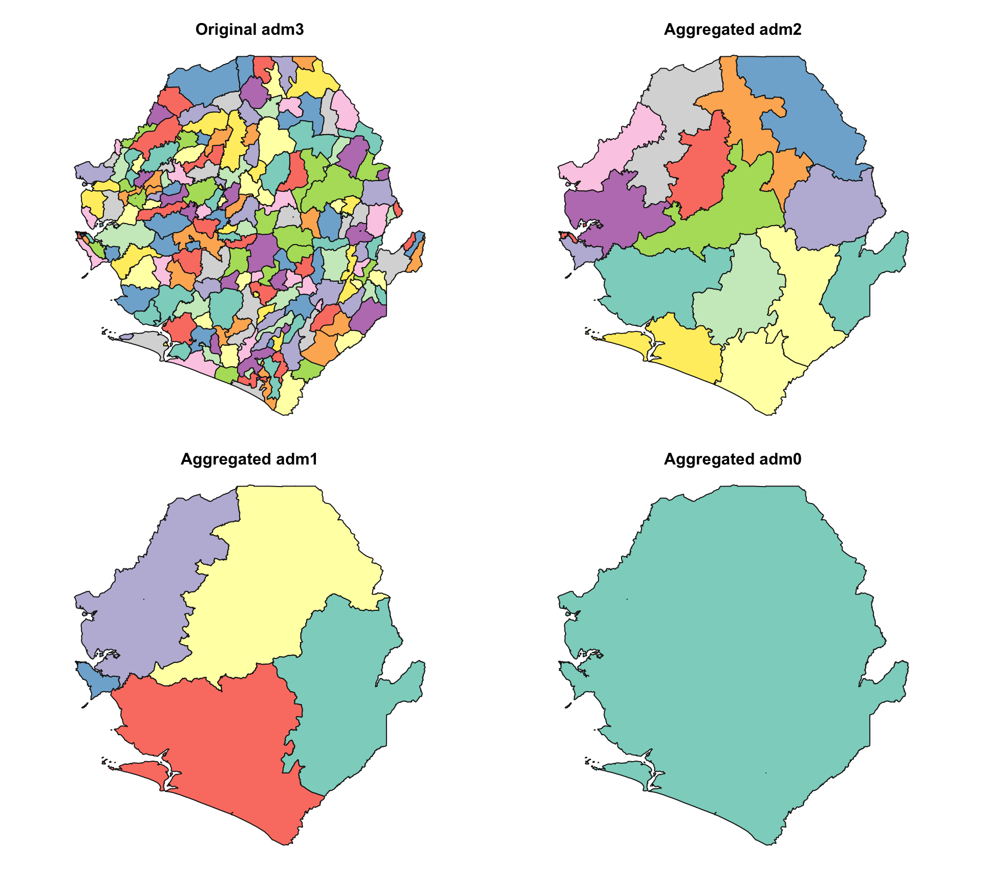
plot(shp_adm3$geometry, col = plot_col, main = "Original adm3")
plot(shp_adm2$geometry, col = plot_col, main = "Aggregated adm2 (from adm3)")
plot(shp_adm1$geometry, col = plot_col, main = "Aggregated adm1 (from adm3)")
plot(shp_adm0$geometry, col = plot_col, main = "Aggregated adm0 (from adm3)")

# reset plotting layout (optional)
graphics::par(mfrow = c(1, 1))

Output

To adapt the code:

Lines 3, 10, and 16: Replace shp_adm3 with the relevant shapefile object.
Lines 4, 11–12, and 17–18: Update the column names (adm0, adm1, adm2) to match those in the data.
Lines 4, 11–12, and 17–18: Adjust the grouping level depending on which higher admin level to create.

Show the code

# create adm0-level shapefile by
# grouping over the country name
shp_adm0 = shp_adm3[["adm0", "geometry"]].dissolve(
    by="adm0",
    as_index=False
)

# create adm1-level shapefile by
# grouping over the region (e.g., province)
shp_adm1 = shp_adm3[["adm0", "adm1", "geometry"]].dissolve(
    by=["adm0", "adm1"],
    as_index=False
)

# create adm2-level shapefile (e.g., districts)
shp_adm2 = shp_adm3[["adm0", "adm1", "adm2", "geometry"]].dissolve(
    by=["adm0", "adm1", "adm2"],
    as_index=False
)

# Check to see the operations worked
# set up a 2x2 plotting area
fig, axes = plt.subplots(2, 2, figsize=(10, 9))
plt.subplots_adjust(
    left=0.01,
    right=0.99,
    bottom=0.01,
    top=0.95,
    wspace=0.02,
    hspace=0.08
)

# set colors
plot_col = sf_colors(208)

# plot each administrative level
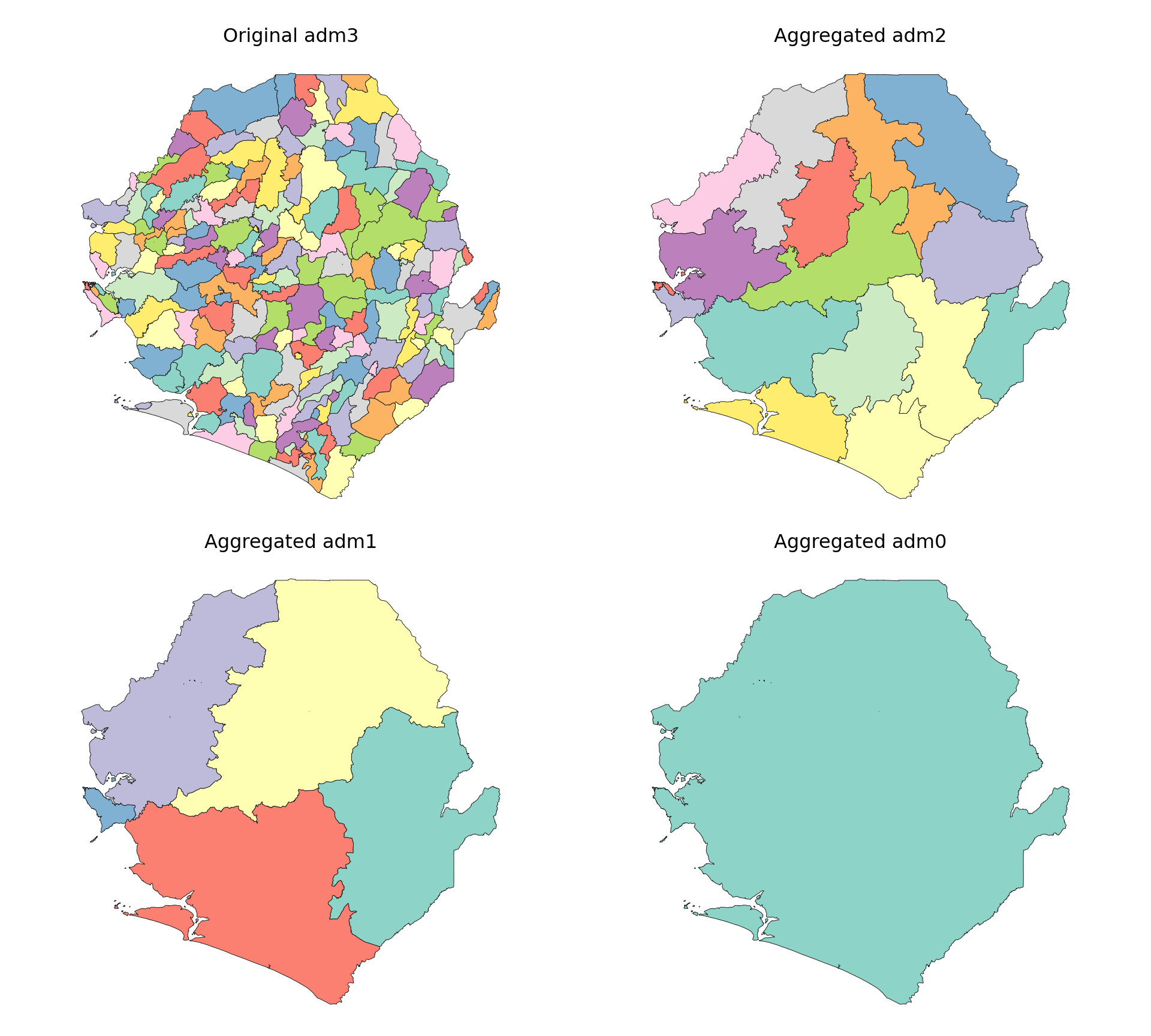
plot_sf_like(shp_adm3, ax=axes[0, 0], colors=plot_col, border="grey10",
             title="Original adm3")
plot_sf_like(shp_adm2, ax=axes[0, 1], colors=plot_col, border="grey10",
             title="Aggregated adm2")
plot_sf_like(shp_adm1, ax=axes[1, 0], colors=plot_col, border="grey10",
             title="Aggregated adm1")
plot_sf_like(shp_adm0, ax=axes[1, 1], colors=plot_col, border="grey10",
             title="Aggregated adm0")

plt.show()

Output

To adapt the code:

Lines 3, 10, and 17: Replace shp_adm3 with the relevant shapefile object.
Lines 3, 10–11, and 17–18: Update the column names (adm0, adm1, adm2) to match those in the data.
Adjust the grouping columns depending on which higher admin level is needed.
Keep sf_colors(...) to match the Python plot colours to the R sf::sf.colors(..., categorical = TRUE) output.

The plots confirm that aggregation to adm0, adm1, and adm2 levels worked as expected. Each map shows progressively coarser boundaries, and the original adm3 structure is preserved.

Step 5: Shapefile customization

Step 5.1: Mixed-level shapefiles

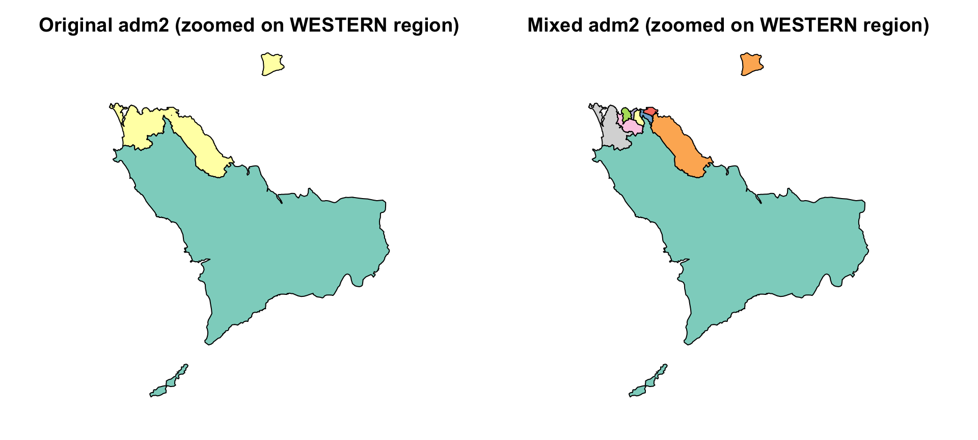
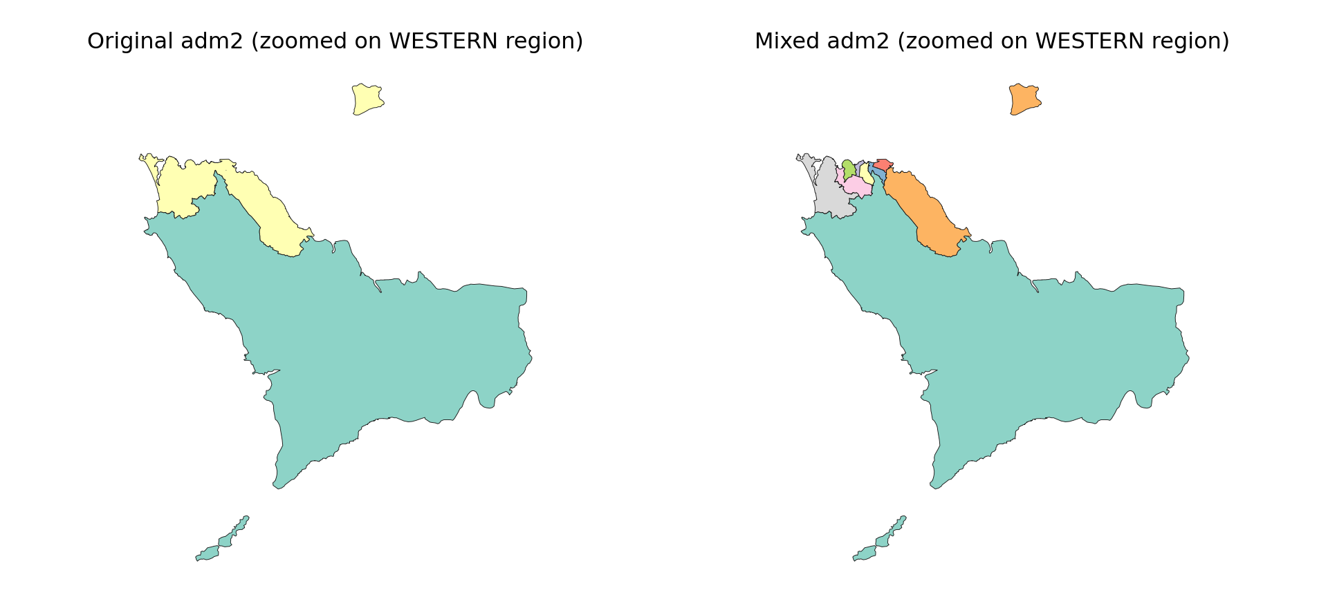
In some cases, we may want to combine different administrative levels within a single shapefile, for example, using adm2 for most of the country while substituting finer adm3 boundaries in selected areas. This approach is useful when certain districts require more granularity for analysis, planning, or visualization, but a full switch to adm3 isn’t necessary.

One use case for this approach is when finer geographic detail is needed only in specific parts of the country. For example, in Sierra Leone, we may want to use adm3 boundaries within Western Area Urban, which includes Freetown, a densely populated area, while retaining adm2 boundaries for the rest of the country. This allows us to maintain national coverage at a manageable resolution, while zooming in where more granularity is required.

Show the code

# remove target adm2 unit from adm2 shapefile
target_adm2 <- "WESTERN URBAN"

adm2_trimmed <- shp_adm2 |>
  dplyr::filter(adm2 != target_adm2)

# get the equivalent adm3 units
adm3_subset <- shp_adm3 |>
  dplyr::filter(adm2 == target_adm2)

# optional: add a column to indicate source level
adm2_trimmed <- adm2_trimmed |> dplyr::mutate(source = "adm2")
adm3_subset <- adm3_subset |> dplyr::mutate(source = "adm3")

# combine them into a single shapefile
shp_mixed <- dplyr::bind_rows(adm2_trimmed, adm3_subset)

# Check to see the operations worked
# set up a 1x2 plotting area
graphics::par(mfrow = c(1, 2))

# set colors
plot_col <- sf::sf.colors(208, categorical = TRUE)

# plot WESTERN to show the finer changes
shp_adm2 |>
  dplyr::filter(adm1 == "WESTERN") |>
  sf::st_geometry() |>
  plot(col = plot_col, main = "Original adm2 (zoomed on WESTERN region)")

shp_mixed |>
  dplyr::filter(adm1 == "WESTERN") |>
  sf::st_geometry() |>
  plot(col = plot_col, main = "Mixed adm2 (zoomed on WESTERN region)")


# reset plotting layout (optional)
graphics::par(mfrow = c(1, 1))

Output

To adapt the code:

To apply this in another context:

Line 2: Replace WESTERN URBAN with the name of the admin unit to swap.
Lines 4–5, 8–9: Update adm2 and adm3 column names if the shapefile uses different labels.
Repeat entire code block as needed for all areas of interest.

Show the code

# remove target adm2 unit from adm2 shapefile
target_adm2 = "WESTERN URBAN"

adm2_trimmed = shp_adm2.loc[shp_adm2["adm2"] != target_adm2].copy()

# get the equivalent adm3 units
adm3_subset = shp_adm3.loc[shp_adm3["adm2"] == target_adm2].copy()

# optional: add a column to indicate source level
adm2_trimmed["source"] = "adm2"
adm3_subset["source"] = "adm3"

# combine them into a single shapefile
shp_mixed = gpd.GeoDataFrame(
    pd.concat([adm2_trimmed, adm3_subset], ignore_index=True, sort=False),
    geometry="geometry",
    crs=shp_adm2.crs
)

# Check to see the operations worked
# set up a 1x2 plotting area
fig, axes = plt.subplots(1, 2, figsize=(10, 4.5))
plt.subplots_adjust(
    left=0.01,
    right=0.99,
    bottom=0.02,
    top=0.90,
    wspace=0.02
)

# set colors
plot_col = sf_colors(208)

# Plot WESTERN to show the finer changes
plot_sf_like(
    shp_adm2.loc[shp_adm2["adm1"] == "WESTERN"],
    ax=axes[0],
    colors=plot_col,
    title="Original adm2 (zoomed on WESTERN region)"
)

plot_sf_like(
    shp_mixed.loc[shp_mixed["adm1"] == "WESTERN"],
    ax=axes[1],
    colors=plot_col,
    title="Mixed adm2 (zoomed on WESTERN region)"
)

plt.show()

Output

To adapt the code:

Line 2: Replace WESTERN URBAN with the name of the admin unit to swap.
Lines 4–5 and 8–9: Update adm2 and adm3 column names if the shapefile uses different labels.
Lines 12–13: Update the source values to use different labels for the mixed-level layer.
Repeat the same pattern for each area where one admin level should be replaced by a finer admin level.

The results show that the operation worked: in the WESTERN region, Western Rural remains as a single adm2 unit, while Western Urban has been successfully replaced by several finer adm3 units. This zoomed view shows differences not visible at the national scale. While shp_mixed includes all regions, this comparison confirms the targeted substitution.

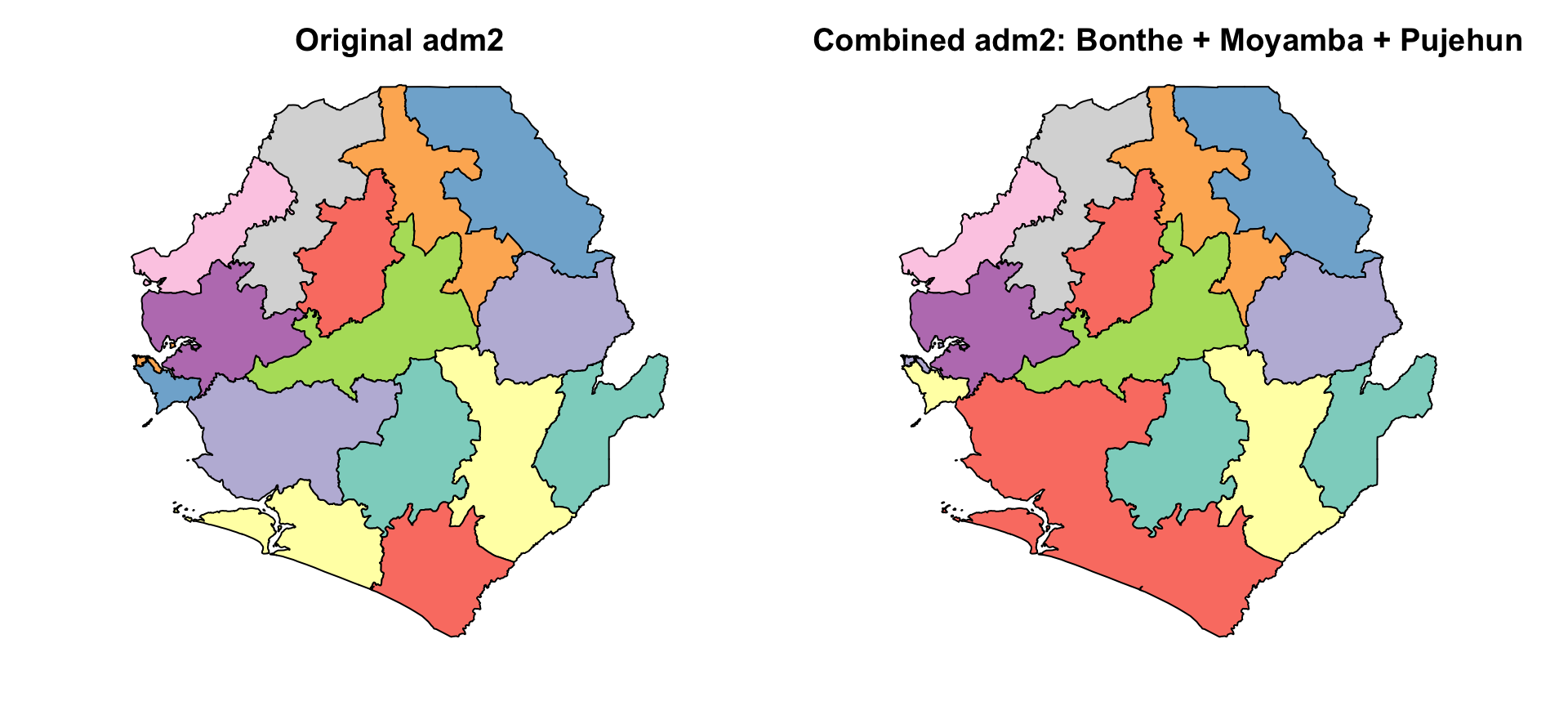
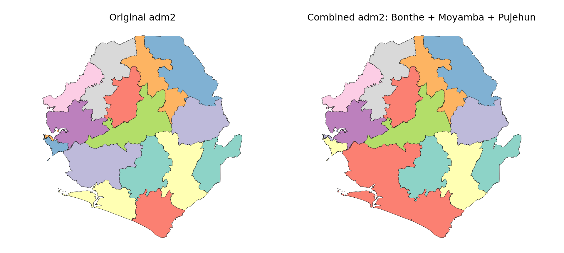
Step 5.2: Merging multiple polygons into a single unit

In some cases, it may be necessary to merge two or more adjacent administrative units into a single geographic feature. This could be done for operational convenience, reporting simplicity, or when small neighboring units should be treated as one planning zone.

For example, we show how three southern districts in Sierra Leone (Bonthe, Moyamba, and Pujehun) can be combined into a single unit.

Show the code

# define the adm2 units to combine
combine_names <- c("BONTHE", "MOYAMBA", "PUJEHUN")

# create a new combined unit
combined <- shp_adm2 |>
  dplyr::filter(adm2 %in% combine_names) |>
  dplyr::summarise(
    adm3 = paste(combine_names, collapse = " ~ "),
    geometry = sf::st_union(geometry),
    .groups = "drop"
  )

# drop the originals and bind the new unit
shp_adm2_combined <- shp_adm2 |>
  dplyr::filter(!adm2 %in% combine_names) |>
  dplyr::bind_rows(combined)

# check to see the operations worked
# set up a 1x2 plotting area
graphics::par(mfrow = c(1, 2))

# set colors
plot_col <- sf::sf.colors(10, categorical = TRUE)

# plot each administrative level
plot(shp_adm2$geometry, col = plot_col, main = "Original adm2")
plot(
  shp_adm2_combined$geometry,
  col = plot_col,
  main = "Combined adm2: Bonthe + Moyamba + Pujehun"
)

# reset plotting layout (optional)
graphics::par(mfrow = c(1, 1))

Output

To adapt the code:

Line 2: Change the names in combine_names to the units to merge.
Lines 6, 15: Update the adm2 field if the shapefile uses a different name (e.g., district_name).
Line 8: Adjust the output name (adm3 = paste(...)) to reflect how the merged unit should be labeled, e.g., use Southern Cluster instead.
Repeat entire code block as needed for all areas of interest.

Show the code

# define the adm2 units to combine
combine_names = ["BONTHE", "MOYAMBA", "PUJEHUN"]

# create a new combined unit
combined = gpd.GeoDataFrame(
    {
        "adm3": [" ~ ".join(combine_names)],
        "geometry": [
            unary_union(
                shp_adm2.loc[shp_adm2["adm2"].isin(combine_names), "geometry"]
            )
        ],
    },
    geometry="geometry",
    crs=shp_adm2.crs
)

# drop the originals and bind the new unit
shp_adm2_combined = gpd.GeoDataFrame(
    pd.concat(
        [
            shp_adm2.loc[~shp_adm2["adm2"].isin(combine_names)],
            combined,
        ],
        ignore_index=True,
        sort=False
    ),
    geometry="geometry",
    crs=shp_adm2.crs
)

# check to see the operations worked
# set up a 1x2 plotting area
fig, axes = plt.subplots(1, 2, figsize=(10, 4.5))
plt.subplots_adjust(
    left=0.01,
    right=0.99,
    bottom=0.02,
    top=0.90,
    wspace=0.02
)

# set colors
plot_col = sf_colors(10)

# plot each administrative level
plot_sf_like(shp_adm2, ax=axes[0], colors=plot_col, title="Original adm2")
plot_sf_like(
    shp_adm2_combined,
    ax=axes[1],
    colors=plot_col,
    title="Combined adm2: Bonthe + Moyamba + Pujehun"
)

plt.show()

Output

To adapt the code:

Line 2: Change the names in combine_names to the units to merge.
Lines 9 and 25: Update the adm2 field if the shapefile uses a different name, such as district_name.
Line 7: Adjust the output name (" ~ ".join(combine_names)) to reflect how the merged unit should be labelled.
Repeat the same code block as needed for all custom merged units.

The plot shows that the selected districts have been successfully merged into a single polygon, forming a custom geographic unit.

Step 6: Create geographic IDs and compare versions

To track changes in boundary geometry over time or across shapefile versions, we generate a geometry-based hash ID for each polygon. This allows us to detect if a unit has changed spatially, even if its name remains the same. We then use those hashes to compare two versions of the same shapefile and visualize what changed.

Step 6.1: Create geometry hashes

This step is useful for verifying shapefile updates, aligning geographies across years, and making sure historical comparisons are done correctly. We can also use geometry hashes to check for duplicate polygons in the same shapefile (Step 3 above).

Show the code

# create a hash ID for each polygon using its geometry
shp_adm3 <- shp_adm3 |>
  dplyr::mutate(
    geometry_hash = sntutils::vdigest(geometry, algo = "xxhash32")
  ) |>
  dplyr::select(adm0, adm1, adm2, adm3, geometry_hash)

shp_adm2 <- shp_adm2 |>
  dplyr::mutate(
    geometry_hash = sntutils::vdigest(geometry, algo = "xxhash32")
  ) |>
  dplyr::select(adm0, adm1, adm2, geometry_hash)

shp_adm1 <- shp_adm1 |>
  dplyr::mutate(
    geometry_hash = sntutils::vdigest(geometry, algo = "xxhash32")
  ) |>
  dplyr::select(adm0, adm1, geometry_hash)

shp_adm0 <- shp_adm0 |>
  dplyr::mutate(
    geometry_hash = sntutils::vdigest(geometry, algo = "xxhash32")
  ) |>
  dplyr::select(adm0, geometry_hash)

# check uniqueness of each shape hash ID
cli::cli_h2("Checking hash ID uniqueness")

adm0_n <- nrow(shp_adm0)
adm0_unique <- dplyr::n_distinct(shp_adm0$geometry_hash)
cli::cli_alert_info("adm0: {adm0_unique} unique hashes across {adm0_n} rows")

adm1_n <- nrow(shp_adm1)
adm1_unique <- dplyr::n_distinct(shp_adm1$geometry_hash)
cli::cli_alert_info("adm1: {adm1_unique} unique hashes across {adm1_n} rows")

adm2_n <- nrow(shp_adm2)
adm2_unique <- dplyr::n_distinct(shp_adm2$geometry_hash)
cli::cli_alert_info("adm2: {adm2_unique} unique hashes across {adm2_n} rows")

adm3_n <- nrow(shp_adm3)
adm3_unique <- dplyr::n_distinct(shp_adm3$geometry_hash)
cli::cli_alert_info("adm3: {adm3_unique} unique hashes across {adm3_n} rows")

# check output
head(shp_adm3)

Output

── Checking hash ID uniqueness ──

ℹ adm0: 1 unique hashes across 1 rows

ℹ adm1: 5 unique hashes across 5 rows

ℹ adm2: 16 unique hashes across 16 rows

ℹ adm3: 208 unique hashes across 208 rows

adm0	adm1	adm2	adm3	geometry_hash	geometry
SIERRA LEONE	EASTERN	KAILAHUN	DEA	bee1a2ea	MULTIPOLYGON (((-10.66064 8…
SIERRA LEONE	EASTERN	KAILAHUN	JAHN	c54ea6d9	MULTIPOLYGON (((-10.90291 8…
SIERRA LEONE	EASTERN	KAILAHUN	JAWIE	d2a4880e	MULTIPOLYGON (((-10.8085 8….
SIERRA LEONE	EASTERN	KAILAHUN	KISSI KAMA	ec4698b1	MULTIPOLYGON (((-10.35988 8…
SIERRA LEONE	EASTERN	KAILAHUN	KISSI TENG	3c531939	MULTIPOLYGON (((-10.31537 8…
SIERRA LEONE	EASTERN	KAILAHUN	KISSI TONGI	fca31da6	MULTIPOLYGON (((-10.27296 8…

To adapt the code:

Lines 2, 8, 14, and 20: Replace shp_adm3, shp_adm2, etc. with the relevant shapefile objects.
Ensure each layer has a geometry column of class sfc.
Lines 6, 12, 18, and 24: The field names (adm0, adm1, etc.) can be adjusted to match the naming scheme in use.

Show the code

# create a hash ID for each polygon using its geometry
shp_adm3 = (
    shp_adm3.assign(
        geometry_hash=shp_adm3.geometry.apply(lambda x: geometry_hash(x, "xxhash32"))
    )
    [["adm0", "adm1", "adm2", "adm3", "geometry_hash", "geometry"]]
)

shp_adm2 = (
    shp_adm2.assign(
        geometry_hash=shp_adm2.geometry.apply(lambda x: geometry_hash(x, "xxhash32"))
    )
    [["adm0", "adm1", "adm2", "geometry_hash", "geometry"]]
)

shp_adm1 = (
    shp_adm1.assign(
        geometry_hash=shp_adm1.geometry.apply(lambda x: geometry_hash(x, "xxhash32"))
    )
    [["adm0", "adm1", "geometry_hash", "geometry"]]
)

shp_adm0 = (
    shp_adm0.assign(
        geometry_hash=shp_adm0.geometry.apply(lambda x: geometry_hash(x, "xxhash32"))
    )
    [["adm0", "geometry_hash", "geometry"]]
)

# Check uniqueness of each shape hash ID
cli_header("Checking hash ID uniqueness")

adm0_n = len(shp_adm0)
adm0_unique = shp_adm0["geometry_hash"].nunique()
cli_info(f"adm0: {adm0_unique} unique hashes across {adm0_n} rows")

adm1_n = len(shp_adm1)
adm1_unique = shp_adm1["geometry_hash"].nunique()
cli_info(f"adm1: {adm1_unique} unique hashes across {adm1_n} rows")

adm2_n = len(shp_adm2)
adm2_unique = shp_adm2["geometry_hash"].nunique()
cli_info(f"adm2: {adm2_unique} unique hashes across {adm2_n} rows")

adm3_n = len(shp_adm3)
adm3_unique = shp_adm3["geometry_hash"].nunique()
cli_info(f"adm3: {adm3_unique} unique hashes across {adm3_n} rows")

# check output
shp_adm3.head()

Output


Checking hash ID uniqueness

INFO: adm0: 1 unique hashes across 1 rows

INFO: adm1: 5 unique hashes across 5 rows

INFO: adm2: 16 unique hashes across 16 rows

INFO: adm3: 208 unique hashes across 208 rows

adm0	adm1	adm2	adm3	geometry_hash
SIERRA LEONE	EASTERN	KAILAHUN	DEA	2b54c620
SIERRA LEONE	EASTERN	KAILAHUN	JAHN	6de64368
SIERRA LEONE	EASTERN	KAILAHUN	JAWIE	ac9a2dde
SIERRA LEONE	EASTERN	KAILAHUN	KISSI KAMA	980f7259
SIERRA LEONE	EASTERN	KAILAHUN	KISSI TENG	71af27e5

To adapt the code:

Lines 2, 9, 16, and 23: Replace shp_adm3, shp_adm2, etc. with the relevant shapefile objects.
Ensure each layer has a valid geometry column.
Lines 6, 13, 20, and 27: Adjust the selected field names (adm0, adm1, etc.) to match the naming scheme in use.
Keep the same hash algorithm across all layers and all shapefile versions that need to be compared.

We now have clean shapefiles for each admin level (adm0–adm3), each tagged with a geometry-based hash ID.

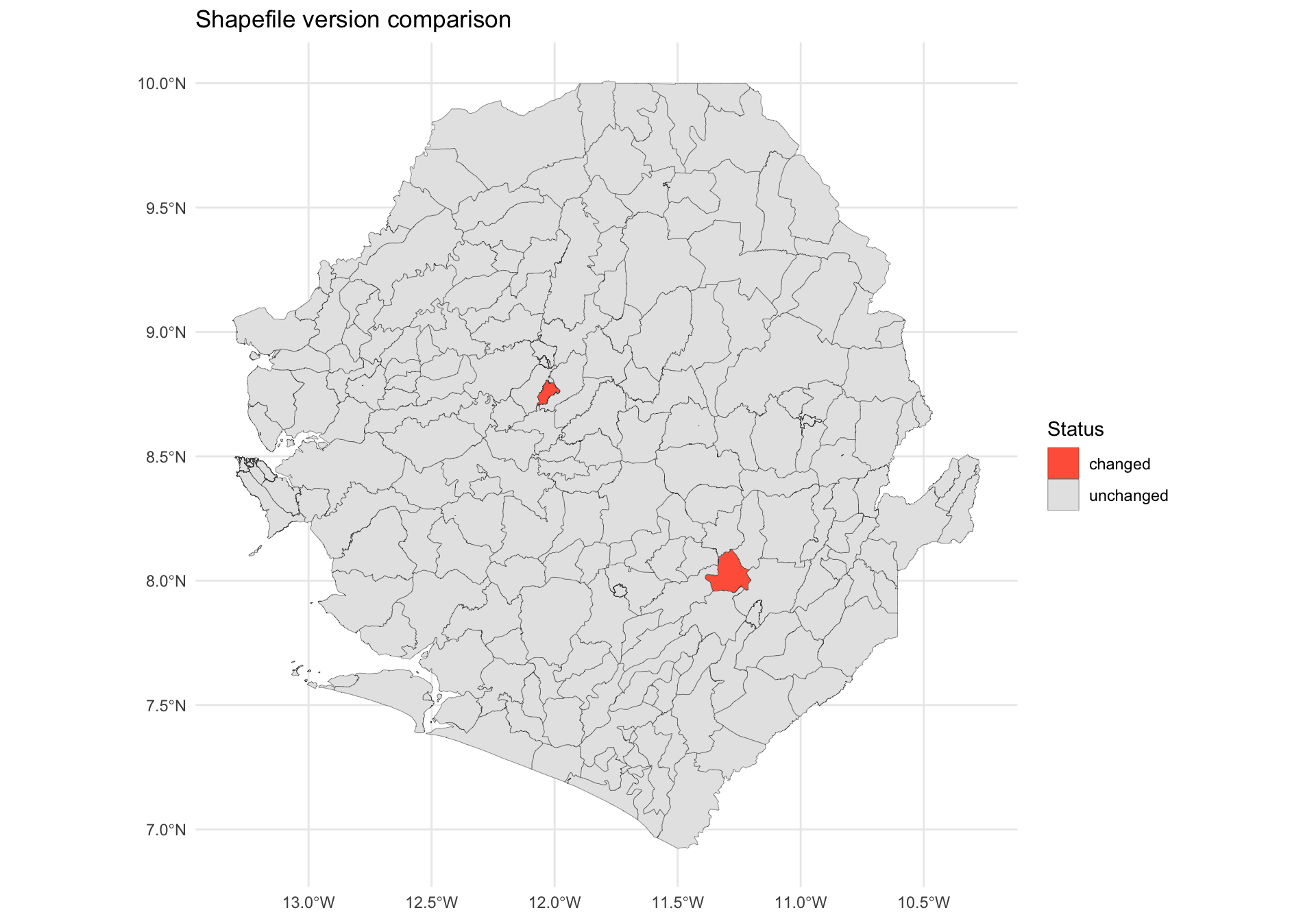
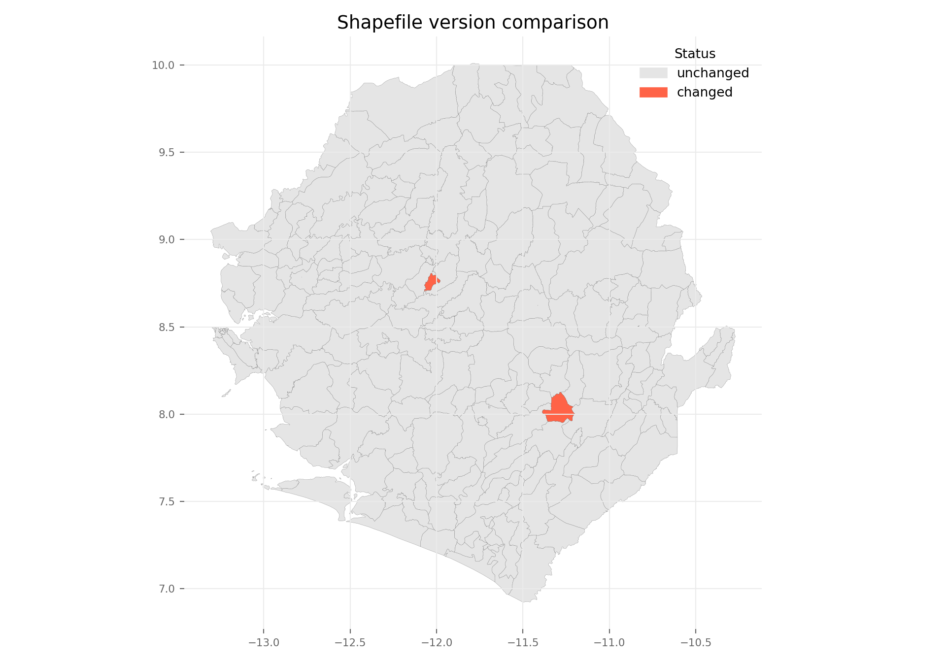
Step 6.2: Compare two shapefile versions visually

Once each polygon has a geometry hash, we can compare a previous version of the shapefile against the current one to see exactly which units changed. We join the two versions by their admin-name keys, classify each unit as unchanged, changed, new, or removed, and overlay the result on a map.

For this demo, we simulate a “previous version” (shp_adm3_v0) by perturbing a few polygons of the current shp_adm3. In real use, shp_adm3_v0 would be loaded from a separately-stored older shapefile.

Show the code

# load the previous version (here we simulate it from shp_adm3)
shp_adm3_v0 <- shp_adm3 |>
  # perturb the geometry of two chiefdoms to simulate boundary redraws
  dplyr::mutate(
    geometry = ifelse(
      seq_len(dplyr::n()) %in% c(20, 50),
      sf::st_buffer(geometry, dist = 0.01),
      geometry
    )
  ) |>
  sf::st_as_sf() |>
  dplyr::mutate(
    geometry_hash = sntutils::vdigest(geometry, algo = "xxhash32")
  )

# join the two versions on the admin-name keys and compare hashes
join_keys <- c("adm0", "adm1", "adm2", "adm3")

diff_df <- shp_adm3 |>
  sf::st_drop_geometry() |>
  dplyr::full_join(
    shp_adm3_v0 |> sf::st_drop_geometry(),
    by = join_keys,
    suffix = c("_new", "_old")
  ) |>
  dplyr::mutate(
    status = dplyr::case_when(
      is.na(geometry_hash_old) ~ "new",
      is.na(geometry_hash_new) ~ "removed",
      geometry_hash_new != geometry_hash_old ~ "changed",
      TRUE ~ "unchanged"
    )
  )

# attach status back to the current version and plot
shp_adm3_diff <- shp_adm3 |>
  dplyr::left_join(
    diff_df |> dplyr::select(dplyr::all_of(join_keys), status),
    by = join_keys
  )

ggplot2::ggplot(shp_adm3_diff) +
  ggplot2::geom_sf(ggplot2::aes(fill = status), colour = "grey30", size = 0.1) +
  ggplot2::scale_fill_manual(values = c(
    unchanged = "grey90",
    changed = "tomato",
    new = "skyblue",
    removed = "orange"
  )) +
  ggplot2::labs(
    title = "Shapefile version comparison",
    fill = "Status"
  ) +
  ggplot2::theme_minimal()

Output

To adapt the code:

Line 2: Replace the simulated shp_adm3_v0 with the actual previous shapefile, loaded via sf::read_sf() and processed through Steps 2–6.1 to attach geometry hashes.
Line 16: Update join_keys to match the admin-name columns in the data.
Lines 40–47: Adjust the colour palette and labels to match the report style.
The same pattern works for higher admin levels by substituting shp_adm2, shp_adm1, etc.

Show the code

# load the previous version (here we simulate it from shp_adm3)
shp_adm3_v0 = shp_adm3.copy()

# perturb the geometry of two chiefdoms to simulate boundary redraws
rows_to_change = shp_adm3_v0.index[[19, 49]]
shp_adm3_v0.loc[rows_to_change, "geometry"] = (
    shp_adm3_v0.loc[rows_to_change, "geometry"].buffer(0.01)
)

shp_adm3_v0 = shp_adm3_v0.assign(
    geometry_hash=shp_adm3_v0.geometry.apply(lambda x: geometry_hash(x, "xxhash32"))
)

# join the two versions on the admin-name keys and compare hashes
join_keys = ["adm0", "adm1", "adm2", "adm3"]

diff_df = (
    shp_adm3.drop(columns="geometry")
    .merge(
        shp_adm3_v0.drop(columns="geometry"),
        on=join_keys,
        how="outer",
        suffixes=("_new", "_old")
    )
)

diff_df["status"] = np.select(
    [
        diff_df["geometry_hash_old"].isna(),
        diff_df["geometry_hash_new"].isna(),
        diff_df["geometry_hash_new"] != diff_df["geometry_hash_old"],
    ],
    ["new", "removed", "changed"],
    default="unchanged"
)

# attach status back to the current version and plot
shp_adm3_diff = shp_adm3.merge(
    diff_df[join_keys + ["status"]],
    on=join_keys,
    how="left"
)

status_colors = {
    "unchanged": "grey90",
    "changed": "tomato",
    "new": "skyblue",
    "removed": "orange",
}

fig, ax = plt.subplots(figsize=(10, 7))
for status, color in status_colors.items():
    subset = shp_adm3_diff.loc[shp_adm3_diff["status"] == status]
    if not subset.empty:
        subset.plot(
            ax=ax,
            color=r_color(color),
            edgecolor=r_color("grey30"),
            linewidth=0.1,
        )

legend_handles = [
    mpatches.Patch(color=r_color(color), label=status)
    for status, color in status_colors.items()
    if status in set(shp_adm3_diff["status"].dropna())
]
ax.legend(handles=legend_handles, title="Status", frameon=False)
ax.set_title("Shapefile version comparison", fontsize=14)
ax.grid(True, color="#ebebeb", linewidth=0.8)
ax.tick_params(labelsize=8, colors="#666666")
for spine in ax.spines.values():
    spine.set_visible(False)
plt.tight_layout()
plt.show()

Output

To adapt the code:

Line 2: Replace the simulated shp_adm3_v0 with the actual previous shapefile, loaded with gpd.read_file() and processed through Steps 2–6.1 to attach geometry hashes.
Line 14: Update join_keys to match the admin-name columns in the data.
Lines 39–44: Adjust the colour palette and labels to match the report style.
The same pattern works for higher admin levels by substituting shp_adm2, shp_adm1, etc.

The map highlights the two perturbed chiefdoms in red (changed), with the rest of the country shown as unchanged. In a real comparison, new units would appear where the newer shapefile added a polygon (e.g., a district split) and removed units where a polygon was retired. This visual diff is faster than reviewing attribute tables row by row and makes it easy to flag affected areas for the SNT team.

Step 7: Saving vector data

After cleaning and transforming spatial data, it is important to save it in a format that preserves the geometry, structure, and CRS. R supports multiple vector formats, and we do not need to use all of them; simply choose the formats that fit the workflow and how the data will be reused or shared.

Below are the main options, with notes on when and how to use them. Use the one(s) that work best for the team and context.

Show the code

# save adm0
saveRDS(
  shp_adm0,
  here::here(
    spat_path, "processed", "sle_spatial_adm0_2021.rds"
  )
)

# save adm1
saveRDS(
  shp_adm1,
  here::here(
    spat_path, "processed", "sle_spatial_adm1_2021.rds"
  )
)

# save adm2
saveRDS(
  shp_adm2,
  here::here(
    spat_path, "processed", "sle_spatial_adm2_2021.rds"
  )
)

# save adm3
saveRDS(
  shp_adm3,
  here::here(
    spat_path, "processed", "sle_spatial_adm3_2021.rds"
  )
)

The example above shows how to save shapefiles of multiple administrative levels using both RDS and st_write functions. Choose the format that best fits the workflow, whether storing layers together or exporting them individually.

If the spatial object was saved using saveRDS(), we can load it with readRDS() and convert it to an sf object:

readRDS(
  here::here(
    "01_data/1.1_foundational/1.1a_admin_boundaries/processed",
    "sle_spatial_adm3_2021.rds"
  )
) |>
  sf::st_as_sf()

GeoJSON (.geojson): For GeoJSON files:

sf::st_write(
  shp_adm3,                                       # object to write
  here::here("folder", "boundary.geojson"),       # output file path
  delete_dsn = TRUE,                              # overwrite file if it exists
  quiet = TRUE                                    # hide write messages
)

GeoPackage (.gpkg): For GeoPackage files:

sf::st_write(
  shp_adm3,                                       # object to write
  here::here("folder", "boundary.gpkg"),          # output file path
  layer = "adm3",                                 # layer name inside gpkg
  delete_layer = TRUE,                            # overwrite layer if it exists
  quiet = TRUE                                    # hide write messages
)

File Geodatabase (.gdb): For Geodatabase files:

sf::st_write(
  shp_adm3,                                       # object to write
  here::here("folder", "boundary.gdb"),           # output geodatabase path
  layer = "adm3",                                 # layer name inside gdb
  driver = "FileGDB",                             # use FileGDB driver
  delete_layer = TRUE,                            # overwrite layer if it exists
  quiet = TRUE                                    # hide write messages
)

To adapt the code:

Lines 2–4, 7–10, 13–16, and 19–22: Adapt the file paths and column names (adm0, adm1, adm2, adm3) based on the relevant folder structure and country-specific data. Not all countries use an adm3 level, so this will vary depending on context.
Choose the format that best fits the workflow: RDS for native R reuse, GeoJSON for broad compatibility, GeoPackage for multi-layer spatial files, or File Geodatabase for ArcGIS pipelines.
Use readRDS() followed by sf::st_as_sf() to load a spatial object previously saved with saveRDS().

Python does not write native R .rds files. For a Python workflow, use open spatial formats such as GeoJSON or GeoPackage, or use GeoParquet for efficient Python-to-Python reuse. If the downstream workflow specifically requires .rds, save that copy from R.

Show the code

processed_path = Path(spat_path) / "processed"
processed_path.mkdir(parents=True, exist_ok=True)

# save adm0
shp_adm0.to_file(
    processed_path / "sle_spatial_adm0_2021.geojson",
    driver="GeoJSON"
)

# save adm1
shp_adm1.to_file(
    processed_path / "sle_spatial_adm1_2021.geojson",
    driver="GeoJSON"
)

# save adm2
shp_adm2.to_file(
    processed_path / "sle_spatial_adm2_2021.geojson",
    driver="GeoJSON"
)

# save adm3
shp_adm3.to_file(
    processed_path / "sle_spatial_adm3_2021.geojson",
    driver="GeoJSON"
)

GeoJSON (.geojson): For GeoJSON files:

shp_adm3.to_file(
    here("folder/boundary.geojson"),       # output file path
    driver="GeoJSON"
)

GeoPackage (.gpkg): For GeoPackage files:

shp_adm3.to_file(
    here("folder/boundary.gpkg"),          # output file path
    layer="adm3",                          # layer name inside gpkg
    driver="GPKG"
)

GeoParquet (.parquet): For efficient Python workflows:

shp_adm3.to_parquet(
    here("folder/boundary.parquet")        # output file path
)

File Geodatabase (.gdb): For Geodatabase files, driver support depends on the local GDAL installation:

shp_adm3.to_file(
    here("folder/boundary.gdb"),           # output geodatabase path
    layer="adm3",                          # layer name inside gdb
    driver="OpenFileGDB"                   # or "FileGDB" if available
)

To adapt the code:

Lines 1–2: Update processed_path to match the project folder structure.
Lines 5, 11, 17, and 23: Replace the object names (shp_adm0, shp_adm1, etc.) if the workflow uses different variable names.
Update output filenames to match the country code, admin level, and boundary year.
Use GeoJSON for broad compatibility, GeoPackage for multi-layer spatial files, or GeoParquet for efficient Python workflows.
If another part of the SNT workflow requires .rds, create that file from the R tab rather than Python.

SNT shapefile QA checklist

Before moving on to any downstream analysis, confirm the cleaned shapefile passes all of the following checks. If any fails, return to the relevant step above.

Valid geometries: sf::st_is_valid() in R, or .geometry.is_valid in Python, returns TRUE/True for every feature (Step 3.1).
Unique polygons: no full-row or geometry-only duplicates remain, using dplyr::distinct()/sf::st_as_binary() in R or .drop_duplicates()/WKB checks in Python (Steps 3.2–3.3).
Consistent CRS: every layer uses the same CRS, typically EPSG:4326, checked with sf::st_crs() in R or .crs in Python (Step 2.2).
No topology errors: no internal gaps or adjacent slivers detected in the R or Python topology summary (Step 3.4).
Aligned admin hierarchy: adm0, adm1, adm2, (and adm3) layers nest cleanly when aggregated with dplyr::summarise()/sf::st_union() in R or .dissolve() in Python (Step 4).
Geometry hash IDs: a unique geometry_hash column is attached to every admin level using sntutils::vdigest() in R or the Python geometry_hash() helper (Step 6.1).
Version-tracked: when an updated shapefile arrives, the diff against the previous version has been reviewed in R or Python (Step 6.2).
Saved durably: the cleaned layers are written to stable formats, such as .rds, .gpkg, or .geojson in R and .geojson, .gpkg, or GeoParquet in Python, with consistent file naming (Step 7).

Keep this checklist alongside the shapefile for each SNT project so the same standards apply to every country and every refresh.

Summary

This section provides a practical foundation for managing shapefile data in the SNT workflow. It walks through the key steps needed to prepare, validate, and customize boundary layers. It offers solutions for resolving geometry issues, handling duplicates, aligning CRS, detecting topology gaps and slivers, and constructing flexible administrative layers tailored to program needs. The page also introduces geometry hashing to support version tracking, demonstrates how to compare and visualize differences between two shapefile versions, and shows how to export cleaned spatial data for analysis and mapping. These steps ensure that all spatial operations in SNT are built on a stable and reproducible geographic base.

Analysts can return to specific steps as needed throughout their work, making this page a long-term reference for consistent spatial data preparation across SNT projects.

Full code

Find the full code script for managing and customising shapefiles below.

Show full code

################################################################################
############# ~ Shapefile management and customization full code ~ #############
################################################################################

### Step 1: Install and load packages ------------------------------------------

# install `pacman` if not already installed
if (!requireNamespace("pacman", quietly = TRUE)) {
  install.packages("pacman")
}

# load required packages using pacman
pacman::p_load(
  sf,         # handling shapefile data
  dplyr,      # data manipulation
  ggplot2,    # plotting
  here,       # file path management
  stringr,    # string manipulation (e.g., str_remove)
  cli,        # clean logging and CLI-style messages
  devtools    # for package management
)

# sntutils has a number of useful helper functions for
# data management and cleaning
if (!requireNamespace("sntutils", quietly = TRUE)) {
  devtools::install_github("ahadi-analytics/sntutils")
}

### Step 2: Load and prepare shapefiles ----------------------------------------

#### Step 2.1: Load and examine data -------------------------------------------

# set up spatial path
spat_path <- here::here(
  "01_data", "1.1_foundational", "1.1a_admin_boundaries"
)

# import shapefile
shp_adm3 <- sf::read_sf(
  here::here(spat_path, "raw", "Chiefdom2021.shp")
) |>
  dplyr::mutate(adm0 = "SIERRA LEONE") |>
  dplyr::select(
    # select relevant columns and rename to standard nomenclature
    adm0,
    adm1 = FIRST_REGI,
    adm2 = FIRST_DNAM,
    adm3 = FIRST_CHIE
  ) |>
  # ensure output remains a valid sf object for downstream usage
  sf::st_as_sf()

# check output by mapping
plot(shp_adm3)

#### Step 2.2: Check and transform CRS -----------------------------------------

cli::cli_h2("Check and assign original CRS for shp_adm3")
shp_adm3 <- sf::st_set_crs(shp_adm3, 4326)
cli::cli_alert_info("Original CRS: {sf::st_crs(shp_adm3)$input}")

# transform to new CRS (e.g., Equal Earth - EPSG:6933)
shp_adm3_diff_crs <- sf::st_transform(shp_adm3, 6933)

cli::cli_h2("Check CRS after transformation")
cli::cli_alert_info("New CRS: {sf::st_crs(shp_adm3_diff_crs)$input}")

### Step 3: Geometry validation ------------------------------------------------

#### Step 3.1: Check and correct geometry validity -----------------------------

# check geometry validity
shp_adm3_inv <- shp_adm3 |>
  dplyr::mutate(
    valid = sf::st_is_valid(geometry),
    invalid_reason = sf::st_is_valid(geometry, reason = TRUE),
    invalid_reason = stringr::str_remove(invalid_reason, "\\[.*")
  )

# get list of invalid adm3s
invalid_df <- shp_adm3_inv |>
  dplyr::filter(!valid) |>
  sf::st_drop_geometry() |>
  dplyr::select(adm0, adm1, adm2, adm3, invalid_reason)

# view invalid rows (if any)
invalid_df

# fix known geometry issues
# (e.g. self-intersections, unclosed rings)
shp_adm3 <- shp_adm3 |>
  sf::st_make_valid()

# re-check and report remaining invalid geometries
n_invalid <- shp_adm3 |>
  dplyr::mutate(valid = sf::st_is_valid(geometry)) |>
  dplyr::filter(!valid) |>
  nrow()

cli::cli_alert_info("Remaining invalid geometries: {n_invalid}")

#### Step 3.2: Check for duplicate polygons ------------------------------------

# check for duplicate geometries
shp_adm3_dup <- shp_adm3 |>
  dplyr::mutate(dup_geom = duplicated(sf::st_as_binary(geometry))) |>
  dplyr::filter(dup_geom == TRUE)

cli::cli_alert_info("Number of duplicated geometries: {nrow(shp_adm3_dup)}")

# check for full row duplicates
dups_full <- shp_adm3 |>
  dplyr::group_by(dplyr::across(dplyr::everything())) |>
  dplyr::filter(dplyr::n() > 1)

# check for geometry-only duplicates
dups_geom <- shp_adm3 |>
  dplyr::mutate(geom_hash = sntutils::vdigest(geometry)) |>
  dplyr::add_count(geom_hash, name = "n_geom") |>
  dplyr::filter(n_geom > 1)

# view results
cli::cli_h1("Checking for full row duplicates")
dups_full |> sf::st_drop_geometry()

cli::cli_h1("Checking for geometry-only duplicates")
dups_geom |> sf::st_drop_geometry()

#### Step 3.3: Resolve any duplicated polygons ---------------------------------

# remove full row duplicates
shp_adm3 <- shp_adm3 |>
  dplyr::distinct()

# if needed, remove known geometry-only duplicates by filtering on labels
# drop intentionally duplicated label
shp_adm3 <- shp_adm3 |>
  dplyr::filter(adm3 != "DUPLICATE LABEL")

# Check  again after cleaning
# check for geometry-only duplicates in shp_adm3
shp_adm3_dup <- shp_adm3 |>
  dplyr::mutate(dup_geom = duplicated(sf::st_as_binary(geometry))) |>
  dplyr::filter(dup_geom == TRUE)

cli::cli_alert_info(
  "Number of duplicated geometries in shp_adm3: {nrow(shp_adm3_dup)}"
)

#### Step 3.4: Check for topology gaps and slivers -----------------------------

# detect adjacent overlaps (slivers) by intersecting the layer with itself
overlaps <- shp_adm3 |>
  sf::st_intersection() |>
  dplyr::filter(n.overlaps > 1) |>
  dplyr::mutate(
    overlap_area_m2 = as.numeric(sf::st_area(geometry))
  ) |>
  # drop true point/line intersections (zero area) and numerical noise
  dplyr::filter(overlap_area_m2 > 1)

cli::cli_alert_info(
  "Adjacent overlap features detected: {nrow(overlaps)}"
)

# detect internal gaps by counting interior rings in the country union.
# use a planar (GEOS) union so the gap count matches the python tab,
# which also unions with GEOS - the spherical s2 union snaps tiny
# slivers differently and reports a different number of holes
s2_was_on <- sf::sf_use_s2()
suppressMessages(sf::sf_use_s2(FALSE))

country_union <- shp_adm3 |>
  sf::st_union() |>
  sf::st_make_valid()

suppressMessages(sf::sf_use_s2(s2_was_on))

# explode the union into individual polygons, then count interior rings
country_polygons <- sf::st_cast(country_union, "POLYGON")

# collect every interior ring as its own polygon
holes <- country_polygons |>
  lapply(\(g) g[-1]) |>
  unlist(recursive = FALSE) |>
  lapply(\(r) sf::st_polygon(list(r)))

# count only holes larger than 1 m2 - sub-metre micro-holes are
# numerical noise whose count varies across geometry engines
hole_areas_m2 <- if (length(holes) == 0) {
  numeric(0)
} else {
  holes |>
    sf::st_sfc(crs = sf::st_crs(country_union)) |>
    sf::st_area() |>
    as.numeric()
}

n_interior_rings <- sum(hole_areas_m2 > 1)

cli::cli_alert_info(
  "Internal gaps (holes inside the country footprint): {n_interior_rings}"
)

# create a visible summary table for the rendered output
topology_summary <- data.frame(
  check = c(
    "Adjacent overlap features detected",
    "Internal gaps (holes inside the country footprint)"
  ),
  count = c(nrow(overlaps), n_interior_rings)
)

topology_summary

### Step 4: Aggregate or reconstruct higher-level administrative boundaries ----

# create adm0-level shapefile by
# grouping over the country name
shp_adm0 <- shp_adm3 |>
  dplyr::group_by(adm0) |>
  dplyr::summarise(.groups = "drop") |>
  sf::st_union(by_feature = TRUE)

# create adm1-level shapefile by
# grouping over the region (e.g., province)
shp_adm1 <- shp_adm3 |>
  dplyr::group_by(adm0, adm1) |>
  dplyr::summarise(.groups = "drop") |>
  sf::st_union(by_feature = TRUE)

# create adm2-level shapefile (e.g., districts)
shp_adm2 <- shp_adm3 |>
  dplyr::group_by(adm0, adm1, adm2) |>
  dplyr::summarise(.groups = "drop") |>
  sf::st_union(by_feature = TRUE)

# Check to see the operations worked
# set up a 2x2 plotting area
graphics::par(mfrow = c(2, 2))

# set colors
plot_col <- sf::sf.colors(208, categorical = TRUE)

# plot each administrative level
plot(shp_adm3$geometry, col = plot_col, main = "Original adm3")
plot(shp_adm2$geometry, col = plot_col, main = "Aggregated adm2 (from adm3)")
plot(shp_adm1$geometry, col = plot_col, main = "Aggregated adm1 (from adm3)")
plot(shp_adm0$geometry, col = plot_col, main = "Aggregated adm0 (from adm3)")

# reset plotting layout (optional)
graphics::par(mfrow = c(1, 1))

### Step 5: Shapefile customization --------------------------------------------

#### Step 5.1: Mixed-level shapefiles ------------------------------------------

# remove target adm2 unit from adm2 shapefile
target_adm2 <- "WESTERN URBAN"

adm2_trimmed <- shp_adm2 |>
  dplyr::filter(adm2 != target_adm2)

# get the equivalent adm3 units
adm3_subset <- shp_adm3 |>
  dplyr::filter(adm2 == target_adm2)

# optional: add a column to indicate source level
adm2_trimmed <- adm2_trimmed |> dplyr::mutate(source = "adm2")
adm3_subset <- adm3_subset |> dplyr::mutate(source = "adm3")

# combine them into a single shapefile
shp_mixed <- dplyr::bind_rows(adm2_trimmed, adm3_subset)

# Check to see the operations worked
# set up a 1x2 plotting area
graphics::par(mfrow = c(1, 2))

# set colors
plot_col <- sf::sf.colors(208, categorical = TRUE)

# plot WESTERN to show the finer changes
shp_adm2 |>
  dplyr::filter(adm1 == "WESTERN") |>
  sf::st_geometry() |>
  plot(col = plot_col, main = "Original adm2 (zoomed on WESTERN region)")

shp_mixed |>
  dplyr::filter(adm1 == "WESTERN") |>
  sf::st_geometry() |>
  plot(col = plot_col, main = "Mixed adm2 (zoomed on WESTERN region)")

# reset plotting layout (optional)
graphics::par(mfrow = c(1, 1))

#### Step 5.2: Merging multiple polygons into a single unit --------------------

# define the adm2 units to combine
combine_names <- c("BONTHE", "MOYAMBA", "PUJEHUN")

# create a new combined unit
combined <- shp_adm2 |>
  dplyr::filter(adm2 %in% combine_names) |>
  dplyr::summarise(
    adm3 = paste(combine_names, collapse = " ~ "),
    geometry = sf::st_union(geometry),
    .groups = "drop"
  )

# drop the originals and bind the new unit
shp_adm2_combined <- shp_adm2 |>
  dplyr::filter(!adm2 %in% combine_names) |>
  dplyr::bind_rows(combined)

# check to see the operations worked
# set up a 1x2 plotting area
graphics::par(mfrow = c(1, 2))

# set colors
plot_col <- sf::sf.colors(10, categorical = TRUE)

# plot each administrative level
plot(shp_adm2$geometry, col = plot_col, main = "Original adm2")
plot(
  shp_adm2_combined$geometry,
  col = plot_col,
  main = "Combined adm2: Bonthe + Moyamba + Pujehun"
)

# reset plotting layout (optional)
graphics::par(mfrow = c(1, 1))

### Step 6: Create geographic IDs and compare versions -------------------------

#### Step 6.1: Create geometry hashes ------------------------------------------

# create a hash ID for each polygon using its geometry
shp_adm3 <- shp_adm3 |>
  dplyr::mutate(
    geometry_hash = sntutils::vdigest(geometry, algo = "xxhash32")
  ) |>
  dplyr::select(adm0, adm1, adm2, adm3, geometry_hash)

shp_adm2 <- shp_adm2 |>
  dplyr::mutate(
    geometry_hash = sntutils::vdigest(geometry, algo = "xxhash32")
  ) |>
  dplyr::select(adm0, adm1, adm2, geometry_hash)

shp_adm1 <- shp_adm1 |>
  dplyr::mutate(
    geometry_hash = sntutils::vdigest(geometry, algo = "xxhash32")
  ) |>
  dplyr::select(adm0, adm1, geometry_hash)

shp_adm0 <- shp_adm0 |>
  dplyr::mutate(
    geometry_hash = sntutils::vdigest(geometry, algo = "xxhash32")
  ) |>
  dplyr::select(adm0, geometry_hash)

# check uniqueness of each shape hash ID
cli::cli_h2("Checking hash ID uniqueness")

adm0_n <- nrow(shp_adm0)
adm0_unique <- dplyr::n_distinct(shp_adm0$geometry_hash)
cli::cli_alert_info("adm0: {adm0_unique} unique hashes across {adm0_n} rows")

adm1_n <- nrow(shp_adm1)
adm1_unique <- dplyr::n_distinct(shp_adm1$geometry_hash)
cli::cli_alert_info("adm1: {adm1_unique} unique hashes across {adm1_n} rows")

adm2_n <- nrow(shp_adm2)
adm2_unique <- dplyr::n_distinct(shp_adm2$geometry_hash)
cli::cli_alert_info("adm2: {adm2_unique} unique hashes across {adm2_n} rows")

adm3_n <- nrow(shp_adm3)
adm3_unique <- dplyr::n_distinct(shp_adm3$geometry_hash)
cli::cli_alert_info("adm3: {adm3_unique} unique hashes across {adm3_n} rows")

# check output
head(shp_adm3)

#### Step 6.2: Compare two shapefile versions visually -------------------------

# load the previous version (here we simulate it from shp_adm3)
shp_adm3_v0 <- shp_adm3 |>
  # perturb the geometry of two chiefdoms to simulate boundary redraws
  dplyr::mutate(
    geometry = ifelse(
      seq_len(dplyr::n()) %in% c(20, 50),
      sf::st_buffer(geometry, dist = 0.01),
      geometry
    )
  ) |>
  sf::st_as_sf() |>
  dplyr::mutate(
    geometry_hash = sntutils::vdigest(geometry, algo = "xxhash32")
  )

# join the two versions on the admin-name keys and compare hashes
join_keys <- c("adm0", "adm1", "adm2", "adm3")

diff_df <- shp_adm3 |>
  sf::st_drop_geometry() |>
  dplyr::full_join(
    shp_adm3_v0 |> sf::st_drop_geometry(),
    by = join_keys,
    suffix = c("_new", "_old")
  ) |>
  dplyr::mutate(
    status = dplyr::case_when(
      is.na(geometry_hash_old) ~ "new",
      is.na(geometry_hash_new) ~ "removed",
      geometry_hash_new != geometry_hash_old ~ "changed",
      TRUE ~ "unchanged"
    )
  )

# attach status back to the current version and plot
shp_adm3_diff <- shp_adm3 |>
  dplyr::left_join(
    diff_df |> dplyr::select(dplyr::all_of(join_keys), status),
    by = join_keys
  )

ggplot2::ggplot(shp_adm3_diff) +
  ggplot2::geom_sf(ggplot2::aes(fill = status), colour = "grey30", size = 0.1) +
  ggplot2::scale_fill_manual(values = c(
    unchanged = "grey90",
    changed = "tomato",
    new = "skyblue",
    removed = "orange"
  )) +
  ggplot2::labs(
    title = "Shapefile version comparison",
    fill = "Status"
  ) +
  ggplot2::theme_minimal()

### Step 7: Saving vector data -------------------------------------------------

# save adm0
saveRDS(
  shp_adm0,
  here::here(
    spat_path, "processed", "sle_spatial_adm0_2021.rds"
  )
)

# save adm1
saveRDS(
  shp_adm1,
  here::here(
    spat_path, "processed", "sle_spatial_adm1_2021.rds"
  )
)

# save adm2
saveRDS(
  shp_adm2,
  here::here(
    spat_path, "processed", "sle_spatial_adm2_2021.rds"
  )
)

# save adm3
saveRDS(
  shp_adm3,
  here::here(
    spat_path, "processed", "sle_spatial_adm3_2021.rds"
  )
)

Show full code

################################################################################
############# ~ Shapefile management and customization full code ~ #############
################################################################################

### Step 1: Install and load packages ------------------------------------------

from pathlib import Path

import geopandas as gpd            # spatial vector data handling
import matplotlib.colors as mcolors
import matplotlib.patches as mpatches
import matplotlib.pyplot as plt    # plotting
import numpy as np                 # conditional logic and arrays
import pandas as pd                # data manipulation
import xxhash                      # fast stable hashing
from pyprojroot import here        # project-relative file paths
from shapely import make_valid
from shapely.geometry import GeometryCollection, MultiPolygon, Polygon
from shapely.ops import unary_union
from shapely.validation import explain_validity

def cli_info(message):
    """Print a simple message similar to cli::cli_alert_info()."""
    print(f"INFO: {message}")

def cli_header(message):
    """Print a simple section header similar to cli::cli_h1()/cli_h2()."""
    print(f"\n{message}")

def cli_success(message):
    """Print a success message similar to cli::cli_alert_success()."""
    print(f"SUCCESS: {message}")

def cli_warning(message):
    """Print a warning message similar to cli::cli_alert_warning()."""
    print(f"WARNING: {message}")

def cli_danger(message):
    """Print an error message similar to cli::cli_alert_danger()."""
    print(f"ERROR: {message}")

def sf_colors(n=10):
    """Match sf::sf.colors(..., categorical = TRUE) using matplotlib palettes."""
    palette_name = "Set2" if n <= 8 else "Set3"
    palette = [mcolors.to_hex(color) for color in plt.get_cmap(palette_name).colors]
    return [palette[i % len(palette)] for i in range(n)]

R_COLOR_MAP = {
    "grey10": "#1a1a1a",
    "gray10": "#1a1a1a",
    "grey30": "#4d4d4d",
    "gray30": "#4d4d4d",
    "grey90": "#e5e5e5",
    "gray90": "#e5e5e5",
}

def r_color(color):
    """Translate common R color names used here into matplotlib colors."""
    return R_COLOR_MAP.get(color, color)

def geometry_wkb(geom):
    """Return WKB bytes for exact-geometry duplicate checks."""
    if geom is None:
        return None
    return geom.wkb

def geometry_hash(geom, algo="xxhash32"):
    """Create a WKB-based geometry hash for duplicate and version checks."""
    if geom is None:
        return None
    payload = geom.wkb
    if algo == "xxhash32":
        return xxhash.xxh32(payload).hexdigest()
    if algo == "xxhash64":
        return xxhash.xxh64(payload).hexdigest()
    raise ValueError("Only xxhash32 and xxhash64 are implemented here.")

def polygonal_part(geom):
    """Keep polygonal output after make_valid() returns a GeometryCollection."""
    if geom is None or geom.is_empty:
        return geom
    if isinstance(geom, (Polygon, MultiPolygon)):
        return geom
    if isinstance(geom, GeometryCollection):
        pieces = [
            part for part in geom.geoms
            if isinstance(part, (Polygon, MultiPolygon))
        ]
        return unary_union(pieces) if pieces else geom
    return geom

def make_valid_polygonal(geom):
    """Python equivalent of sf::st_make_valid() for polygon layers."""
    return polygonal_part(make_valid(geom))

def as_geodataframe(data, crs=None):
    """Coerce a GeoDataFrame, GeoSeries, or geometry list to GeoDataFrame."""
    if isinstance(data, gpd.GeoDataFrame):
        return data
    if isinstance(data, gpd.GeoSeries):
        return gpd.GeoDataFrame(geometry=data, crs=data.crs)
    return gpd.GeoDataFrame(geometry=gpd.GeoSeries(data), crs=crs)

def plot_sf_like(
    data,
    ax=None,
    colors=None,
    border="grey10",
    linewidth=0.35,
    title=None,
    title_size=12,
):
    """Draw a map with styling close to base R sf plotting."""
    gdf = as_geodataframe(data)
    if ax is None:
        _, ax = plt.subplots()

    if colors is None:
        colors = sf_colors(len(gdf))
    elif isinstance(colors, str):
        colors = r_color(colors)
    else:
        colors = [r_color(colors[i % len(colors)]) for i in range(len(gdf))]

    gdf.plot(
        ax=ax,
        color=colors,
        edgecolor=r_color(border) if border else None,
        linewidth=linewidth,
    )
    ax.set_title(title or "", fontsize=title_size)
    ax.set_axis_off()
    ax.set_aspect("equal")
    return ax

### Step 2: Load and prepare shapefiles ----------------------------------------

#### Step 2.1: Load and examine data -------------------------------------------

# set up spatial path
spat_path = here("01_data/1.1_foundational/1.1a_admin_boundaries")

# import shapefile
shp_adm3 = (
    gpd.read_file(Path(spat_path) / "raw" / "Chiefdom2021.shp")
    .assign(adm0="SIERRA LEONE")
    .rename(columns={
        "FIRST_REGI": "adm1",
        "FIRST_DNAM": "adm2",
        "FIRST_CHIE": "adm3",
    })
    [["adm0", "adm1", "adm2", "adm3", "geometry"]]
)

# check output by mapping
ax = plot_sf_like(shp_adm3, title="")
plt.show()

#### Step 2.2: Check and transform CRS -----------------------------------------

cli_header("Check and assign original CRS for shp_adm3")
shp_adm3 = shp_adm3.set_crs(epsg=4326, allow_override=True)
cli_info(f"Original CRS: {shp_adm3.crs}")

# Transform to new CRS (e.g., Equal Earth - EPSG:6933)
shp_adm3_diff_crs = shp_adm3.to_crs(epsg=6933)

cli_header("Check CRS after transformation")
cli_info(f"New CRS: {shp_adm3_diff_crs.crs}")

### Step 3: Geometry validation ------------------------------------------------

#### Step 3.1: Check and correct geometry validity -----------------------------

# check geometry validity
shp_adm3_inv = shp_adm3.copy()
shp_adm3_inv["valid"] = shp_adm3_inv.geometry.is_valid
shp_adm3_inv["invalid_reason"] = (
    shp_adm3_inv.geometry.apply(explain_validity)
    .str.replace(r"\[.*", "", regex=True)
    .str.strip()
)

# get list of invalid adm3s
invalid_df = (
    shp_adm3_inv.loc[~shp_adm3_inv["valid"], [
        "adm0", "adm1", "adm2", "adm3", "invalid_reason"
    ]]
    .reset_index(drop=True)
)

# view invalid rows (if any)
invalid_df

# fix known geometry issues
# (e.g. self-intersections, unclosed rings)
shp_adm3 = shp_adm3.copy()
shp_adm3["geometry"] = shp_adm3.geometry.apply(make_valid_polygonal)

# re-check and report remaining invalid geometries
n_invalid = int((~shp_adm3.geometry.is_valid).sum())

cli_info(f"Remaining invalid geometries: {n_invalid}")

#### Step 3.2: Check for duplicate polygons ------------------------------------

# check for duplicate geometries
shp_adm3_dup = (
    shp_adm3.assign(
        dup_geom=shp_adm3.geometry.apply(geometry_wkb).duplicated()
    )
    .loc[lambda x: x["dup_geom"]]
)

cli_info(f"Number of duplicated geometries: {len(shp_adm3_dup)}")

# Check for full row duplicates
shp_adm3_for_dups = shp_adm3.assign(
    geometry_wkb=shp_adm3.geometry.apply(geometry_wkb)
)

dups_full = (
    shp_adm3_for_dups
    .loc[
        shp_adm3_for_dups.duplicated(
            subset=["adm0", "adm1", "adm2", "adm3", "geometry_wkb"],
            keep=False
        )
    ]
    .drop(columns="geometry_wkb")
)

# Check for geometry-only duplicates
dups_geom = (
    shp_adm3.assign(geom_hash=shp_adm3.geometry.apply(geometry_hash))
    .assign(n_geom=lambda x: x.groupby("geom_hash")["geom_hash"].transform("size"))
    .loc[lambda x: x["n_geom"] > 1]
)

# View results
cli_header("Checking for full row duplicates")
dups_full.drop(columns="geometry")

cli_header("Checking for geometry-only duplicates")
dups_geom.drop(columns="geometry")

#### Step 3.3: Resolve any duplicated polygons ---------------------------------

# remove full row duplicates
shp_adm3 = (
    shp_adm3.assign(geometry_wkb=shp_adm3.geometry.apply(geometry_wkb))
    .drop_duplicates(
        subset=["adm0", "adm1", "adm2", "adm3", "geometry_wkb"]
    )
    .drop(columns="geometry_wkb")
)
shp_adm3 = gpd.GeoDataFrame(shp_adm3, geometry="geometry", crs=shp_adm3.crs)

# if needed, remove known geometry-only duplicates by filtering on labels
# drop intentionally duplicated label
shp_adm3 = shp_adm3.loc[shp_adm3["adm3"] != "DUPLICATE LABEL"].copy()

# Check again after cleaning
# check for geometry-only duplicates in shp_adm3
shp_adm3_dup = (
    shp_adm3.assign(
        dup_geom=shp_adm3.geometry.apply(geometry_wkb).duplicated()
    )
    .loc[lambda x: x["dup_geom"]]
)

cli_info(f"Number of duplicated geometries in shp_adm3: {len(shp_adm3_dup)}")

#### Step 3.4: Check for topology gaps and slivers -----------------------------

# detect adjacent overlaps (slivers) by intersecting the layer with itself
# Use an equal-area CRS for square-metre area calculations.
work = (
    shp_adm3.to_crs(epsg=6933)
    if shp_adm3.crs is not None and shp_adm3.crs.is_geographic
    else shp_adm3.copy()
)

left = (
    work[["geometry"]]
    .reset_index()
    .rename(columns={"index": "left_id"})
)
right = (
    work[["geometry"]]
    .reset_index()
    .rename(columns={"index": "right_id"})
)

intersections = gpd.overlay(
    left,
    right,
    how="intersection",
    keep_geom_type=False
)

overlaps = (
    intersections
    .loc[lambda x: x["left_id"] < x["right_id"]]
    .assign(overlap_area_m2=lambda x: x.geometry.area)
    # drop true point/line intersections (zero area) and numerical noise
    .loc[lambda x: x["overlap_area_m2"] > 1]
)

cli_info(f"Adjacent overlap features detected: {len(overlaps)}")

# detect internal gaps by counting interior rings in the country union
country_union = polygonal_part(make_valid(unary_union(shp_adm3.geometry)))

# explode the union into individual polygons, then count interior rings
if isinstance(country_union, Polygon):
    country_polygons = [country_union]
elif isinstance(country_union, MultiPolygon):
    country_polygons = list(country_union.geoms)
else:
    country_polygons = [
        part for part in country_union.geoms
        if isinstance(part, Polygon)
    ]

# collect every interior ring as its own polygon and count only holes
# larger than 1 m2 - sub-metre micro-holes are numerical noise whose
# count varies across geometry engines
holes = [
    Polygon(ring)
    for poly in country_polygons
    for ring in poly.interiors
]

if holes:
    hole_areas_m2 = (
        gpd.GeoSeries(holes, crs=shp_adm3.crs)
        .to_crs(epsg=6933)
        .area
    )
    n_interior_rings = int((hole_areas_m2 > 1).sum())
else:
    n_interior_rings = 0

cli_info(f"Internal gaps (holes inside the country footprint): {n_interior_rings}")

### Step 4: Aggregate or reconstruct higher-level administrative boundaries ----

# create adm0-level shapefile by
# grouping over the country name
shp_adm0 = shp_adm3[["adm0", "geometry"]].dissolve(
    by="adm0",
    as_index=False
)

# create adm1-level shapefile by
# grouping over the region (e.g., province)
shp_adm1 = shp_adm3[["adm0", "adm1", "geometry"]].dissolve(
    by=["adm0", "adm1"],
    as_index=False
)

# create adm2-level shapefile (e.g., districts)
shp_adm2 = shp_adm3[["adm0", "adm1", "adm2", "geometry"]].dissolve(
    by=["adm0", "adm1", "adm2"],
    as_index=False
)

# Check to see the operations worked
# set up a 2x2 plotting area
fig, axes = plt.subplots(2, 2, figsize=(10, 9))
plt.subplots_adjust(
    left=0.01,
    right=0.99,
    bottom=0.01,
    top=0.95,
    wspace=0.02,
    hspace=0.08
)

# set colors
plot_col = sf_colors(208)

# plot each administrative level
plot_sf_like(shp_adm3, ax=axes[0, 0], colors=plot_col, border="grey10",
             title="Original adm3")
plot_sf_like(shp_adm2, ax=axes[0, 1], colors=plot_col, border="grey10",
             title="Aggregated adm2")
plot_sf_like(shp_adm1, ax=axes[1, 0], colors=plot_col, border="grey10",
             title="Aggregated adm1")
plot_sf_like(shp_adm0, ax=axes[1, 1], colors=plot_col, border="grey10",
             title="Aggregated adm0")

plt.show()

### Step 5: Shapefile customization --------------------------------------------

#### Step 5.1: Mixed-level shapefiles ------------------------------------------

# remove target adm2 unit from adm2 shapefile
target_adm2 = "WESTERN URBAN"

adm2_trimmed = shp_adm2.loc[shp_adm2["adm2"] != target_adm2].copy()

# get the equivalent adm3 units
adm3_subset = shp_adm3.loc[shp_adm3["adm2"] == target_adm2].copy()

# optional: add a column to indicate source level
adm2_trimmed["source"] = "adm2"
adm3_subset["source"] = "adm3"

# combine them into a single shapefile
shp_mixed = gpd.GeoDataFrame(
    pd.concat([adm2_trimmed, adm3_subset], ignore_index=True, sort=False),
    geometry="geometry",
    crs=shp_adm2.crs
)

# Check to see the operations worked
# set up a 1x2 plotting area
fig, axes = plt.subplots(1, 2, figsize=(10, 4.5))
plt.subplots_adjust(
    left=0.01,
    right=0.99,
    bottom=0.02,
    top=0.90,
    wspace=0.02
)

# set colors
plot_col = sf_colors(208)

# Plot WESTERN to show the finer changes
plot_sf_like(
    shp_adm2.loc[shp_adm2["adm1"] == "WESTERN"],
    ax=axes[0],
    colors=plot_col,
    title="Original adm2 (zoomed on WESTERN region)"
)

plot_sf_like(
    shp_mixed.loc[shp_mixed["adm1"] == "WESTERN"],
    ax=axes[1],
    colors=plot_col,
    title="Mixed adm2 (zoomed on WESTERN region)"
)

plt.show()

#### Step 5.2: Merging multiple polygons into a single unit --------------------

# define the adm2 units to combine
combine_names = ["BONTHE", "MOYAMBA", "PUJEHUN"]

# create a new combined unit
combined = gpd.GeoDataFrame(
    {
        "adm3": [" ~ ".join(combine_names)],
        "geometry": [
            unary_union(
                shp_adm2.loc[shp_adm2["adm2"].isin(combine_names), "geometry"]
            )
        ],
    },
    geometry="geometry",
    crs=shp_adm2.crs
)

# drop the originals and bind the new unit
shp_adm2_combined = gpd.GeoDataFrame(
    pd.concat(
        [
            shp_adm2.loc[~shp_adm2["adm2"].isin(combine_names)],
            combined,
        ],
        ignore_index=True,
        sort=False
    ),
    geometry="geometry",
    crs=shp_adm2.crs
)

# check to see the operations worked
# set up a 1x2 plotting area
fig, axes = plt.subplots(1, 2, figsize=(10, 4.5))
plt.subplots_adjust(
    left=0.01,
    right=0.99,
    bottom=0.02,
    top=0.90,
    wspace=0.02
)

# set colors
plot_col = sf_colors(10)

# plot each administrative level
plot_sf_like(shp_adm2, ax=axes[0], colors=plot_col, title="Original adm2")
plot_sf_like(
    shp_adm2_combined,
    ax=axes[1],
    colors=plot_col,
    title="Combined adm2: Bonthe + Moyamba + Pujehun"
)

plt.show()

### Step 6: Create geographic IDs and compare versions -------------------------

#### Step 6.1: Create geometry hashes ------------------------------------------

# create a hash ID for each polygon using its geometry
shp_adm3 = (
    shp_adm3.assign(
        geometry_hash=shp_adm3.geometry.apply(lambda x: geometry_hash(x, "xxhash32"))
    )
    [["adm0", "adm1", "adm2", "adm3", "geometry_hash", "geometry"]]
)

shp_adm2 = (
    shp_adm2.assign(
        geometry_hash=shp_adm2.geometry.apply(lambda x: geometry_hash(x, "xxhash32"))
    )
    [["adm0", "adm1", "adm2", "geometry_hash", "geometry"]]
)

shp_adm1 = (
    shp_adm1.assign(
        geometry_hash=shp_adm1.geometry.apply(lambda x: geometry_hash(x, "xxhash32"))
    )
    [["adm0", "adm1", "geometry_hash", "geometry"]]
)

shp_adm0 = (
    shp_adm0.assign(
        geometry_hash=shp_adm0.geometry.apply(lambda x: geometry_hash(x, "xxhash32"))
    )
    [["adm0", "geometry_hash", "geometry"]]
)

# Check uniqueness of each shape hash ID
cli_header("Checking hash ID uniqueness")

adm0_n = len(shp_adm0)
adm0_unique = shp_adm0["geometry_hash"].nunique()
cli_info(f"adm0: {adm0_unique} unique hashes across {adm0_n} rows")

adm1_n = len(shp_adm1)
adm1_unique = shp_adm1["geometry_hash"].nunique()
cli_info(f"adm1: {adm1_unique} unique hashes across {adm1_n} rows")

adm2_n = len(shp_adm2)
adm2_unique = shp_adm2["geometry_hash"].nunique()
cli_info(f"adm2: {adm2_unique} unique hashes across {adm2_n} rows")

adm3_n = len(shp_adm3)
adm3_unique = shp_adm3["geometry_hash"].nunique()
cli_info(f"adm3: {adm3_unique} unique hashes across {adm3_n} rows")

# check output
shp_adm3.head()

#### Step 6.2: Compare two shapefile versions visually -------------------------

# load the previous version (here we simulate it from shp_adm3)
shp_adm3_v0 = shp_adm3.copy()

# perturb the geometry of two chiefdoms to simulate boundary redraws
rows_to_change = shp_adm3_v0.index[[19, 49]]
shp_adm3_v0.loc[rows_to_change, "geometry"] = (
    shp_adm3_v0.loc[rows_to_change, "geometry"].buffer(0.01)
)

shp_adm3_v0 = shp_adm3_v0.assign(
    geometry_hash=shp_adm3_v0.geometry.apply(lambda x: geometry_hash(x, "xxhash32"))
)

# join the two versions on the admin-name keys and compare hashes
join_keys = ["adm0", "adm1", "adm2", "adm3"]

diff_df = (
    shp_adm3.drop(columns="geometry")
    .merge(
        shp_adm3_v0.drop(columns="geometry"),
        on=join_keys,
        how="outer",
        suffixes=("_new", "_old")
    )
)

diff_df["status"] = np.select(
    [
        diff_df["geometry_hash_old"].isna(),
        diff_df["geometry_hash_new"].isna(),
        diff_df["geometry_hash_new"] != diff_df["geometry_hash_old"],
    ],
    ["new", "removed", "changed"],
    default="unchanged"
)

# attach status back to the current version and plot
shp_adm3_diff = shp_adm3.merge(
    diff_df[join_keys + ["status"]],
    on=join_keys,
    how="left"
)

status_colors = {
    "unchanged": "grey90",
    "changed": "tomato",
    "new": "skyblue",
    "removed": "orange",
}

fig, ax = plt.subplots(figsize=(10, 7))
for status, color in status_colors.items():
    subset = shp_adm3_diff.loc[shp_adm3_diff["status"] == status]
    if not subset.empty:
        subset.plot(
            ax=ax,
            color=r_color(color),
            edgecolor=r_color("grey30"),
            linewidth=0.1,
        )

legend_handles = [
    mpatches.Patch(color=r_color(color), label=status)
    for status, color in status_colors.items()
    if status in set(shp_adm3_diff["status"].dropna())
]
ax.legend(handles=legend_handles, title="Status", frameon=False)
ax.set_title("Shapefile version comparison", fontsize=14)
ax.grid(True, color="#ebebeb", linewidth=0.8)
ax.tick_params(labelsize=8, colors="#666666")
for spine in ax.spines.values():
    spine.set_visible(False)
plt.tight_layout()
plt.show()

### Step 7: Saving vector data -------------------------------------------------

processed_path = Path(spat_path) / "processed"
processed_path.mkdir(parents=True, exist_ok=True)

# save adm0
shp_adm0.to_file(
    processed_path / "sle_spatial_adm0_2021.geojson",
    driver="GeoJSON"
)

# save adm1
shp_adm1.to_file(
    processed_path / "sle_spatial_adm1_2021.geojson",
    driver="GeoJSON"
)

# save adm2
shp_adm2.to_file(
    processed_path / "sle_spatial_adm2_2021.geojson",
    driver="GeoJSON"
)

# save adm3
shp_adm3.to_file(
    processed_path / "sle_spatial_adm3_2021.geojson",
    driver="GeoJSON"
)