# Load required packages
pacman::p_load(
  terra,         # For raster operations
  sf,            # For vector data
  dplyr,         # For data manipulation
  here,          # For file path management
  glue           # For dynamic string construction
)

# Download latest sntutils if you haven't already
devtools::install_github("ahadi-analytics/sntutils")

# Define folder to store IHME surfaces
maps_data_path <- here::here(
  "1.2_epidemiology/1.2c_mortality_estimates/raw"
)

# Load admin boundary shapefile
sle_shp <- readRDS(
  here::here(
    "1.1_foundational/1a_admin_boundaries",
    "1ai_adm3",
    "sle_spatial_adm3_2021.rds"
  )
)Modeled estimates of malaria mortality and proxies
Intermediate
Overview
Reducing malaria deaths is often a primary concern for NMPs, and therefore identifying areas with particularly high malaria mortality is essential in SNT such that they can be prioritized for interventions. Ideally, SNT should use subnational data on malaria mortality of a sufficient quality, granularity, and recency that it can inform decision-making. However, because of weak systems of vital registration and a substantial portion of malaria deaths occurring in the community, accurate malaria mortality data at a granular level is difficult to find, and the SNT team should discuss and identify the best or most appropriate source of malaria mortality data.
In the absence of high-quality data or estimates on malaria-attributable deaths, the SNT team may consider alternate sources of mortality that may serve as a proxy to malaria mortality. All-cause under-5 mortality rate (U5MR) may be considered in areas of high malaria transmission, as malaria is one of the primary causes of death among children under 5. When evaluated, the absolute values (or magnitude) of this indicator may not be directly understood as malaria mortality. Instead, its spatial distribution will be explored, so that areas with higher all-cause U5MR are also considered to be of higher malaria mortality compared to other areas. While U5MR can be estimated from national household surveys, these surveys have limited spatial resolution. Geospatial models can be used to infer U5MR at finer spatial resolution; and the SNT team may wish to engage groups with this type of expertise to conduct this kind of analysis.
In this section, we will explore the all-cause U5MR estimates produced by the Institute for Health Metrics and Evaluation (IHME) that were available in the past. The estimates were made publicly available in the form of raster files that contained pixel-level estimates of U5MR per year between 2000 and 2017. Updated versions are currently under review and not yet available.
NoteObjectives
- Locate and download IHME-modeled U5MR raster datasets
- Extract population-weighted U5MR values at the relevant admin unit level across all available years
- Validate IHME outputs over time and geography
- Finalize cleaned outputs that can be used in SNT analysis
Considerations When Working with IHME Mortality Estimates
The IHME U5MR rasters provide modeled annual probability estimates, expressed as rates per 1,000 live births, for the likelihood of a child dying before age five. These are available at ~5×5 km resolution across 99 low- and middle-income countries for the years 2000 to 2017. While the spatial and temporal consistency of these surfaces makes them a useful input to SNT analyses, several important considerations apply:
1. Modeled estimates, not measured data: The IHME rasters are statistical estimates, not direct measurements. They are produced using Bayesian geostatistical modeling that draws from multiple sources, including surveys, censuses, and covariates. While this allows for full spatial coverage, the surfaces reflect model assumptions and input limitations. They should always be interpreted as modeled approximations, not definitive or authoritative figures.
2. Confidence intervals reflect model uncertainty: Each mortality raster is accompanied by lower and upper bounds, representing the 2.5% and 97.5% quantiles of the posterior distribution. These provide a credible interval around the central estimate and should be used to express uncertainty when reporting or visualizing results. The range between lower and upper bounds can vary by location and year, depending on input data density and model precision.
3. Coverage is historical, not current: These rasters cover the years 2000 to 2017. No IHME mortality surfaces have been released since then. For recent years, you will need to explore other sources or triangulate with other data. The 2000-2017 rasters are most useful for: 1) providing historical context; 2) exploring long-term patterns; and 3) supporting baseline stratification where no better alternative exists.
ImportantConsult SNT Team
Mortality data selection in SNT should not be made in isolation. Whether using national survey estimates, routine health information reporting, or modeled estimates, each source has strengths and limitations.
Best practice is to compile and visualize all available mortality sources for your country or region (e.g. survey, routine, modeled estimate). These should then be reviewed and discussed collectively by the SNT team.
- It is not the analyst’s role to select a single source a priori. The appropriate dataset for decision-making is context-specific and must be agreed upon by the SNT team.
- If unsure, contact the SNT team for support on data quality, triangulation strategies, or how to present alternative mortality estimates for review.
- Ensure that any source used has been formally reviewed and validated before being integrated into subsequent SNT steps.
Even technically sound sources may be inappropriate if they contradict national figures or lack stakeholder consensus. Always consult the SNT team before finalizing mortality inputs.
Step-by-Step
This section guides you through the key steps for accessing, preparing, and extracting U5MR data from IHME raster surfaces. These steps assume you have already reviewed the data considerations and confirmed that IHME is an appropriate source for your context. The goal is to help you generate admin-level estimates, either as rates that can be used in SNT analysis, mapping, or modeling workflows.
The following step-by-step guide will walk you through each stage of the process.
Step 1: Initial Setup, Check and Load IHME Rasters
Step 1.1: Initial setup
In this step, we’ll load the required packages and the shapefile. We’ll use an administrative boundary shapefile for Sierra Leone as an example.
To adapt the code:
- Lines 13–15: Replace the placeholder with the actual directory path where you intend to save your relevant IHME mortality surfaces.
- Lines 18–23: Replace with the path to your shapefile.
Once updated, run the code to load your packages and shapefile.
Step 1.2 Accessing IHME mortality rasters
To work with IHME U5MR data, you’ll first need to download the appropriate raster files from the Global Health Data Exchange (GHDx). Access is free, but a user account is required.
These rasters represent modeled probabilities of death before age five for each 5×5 km pixel, estimated annually from 2000 to 2017. For each year, IHME provides:
- Mean estimates: Central modeled values for U5MR
- Lower bound estimates: Lower 95% uncertainty bound
- Upper bound estimates: Upper 95% uncertainty bound
You will extract all three in later steps to generate a range of estimates at your desired administrative level.
Go to ghdx.healthdata.org
Create a free account or log in.
Go here or search for:
Under-5 mortality rate for low- and middle-income countries 2000-2017Click on the files tab that is just under the page title.
Now download the following rasters:
Under-5 Mortality 2000-2017: Probability of Death, Mean Estimates [GeoTiff]Under-5 Mortality 2000-2017: Probability of Death, Upper Estimates [GeoTiff]Under-5 Mortality 2000-2017: Probability of Death, Lower Estimates [GeoTiff]
- Unzip and save the rasters to your designated path set up in
maps_data_path.
Step 1.3 Import rasters
Once you’ve downloaded and extracted the IHME raster stacks, you can import them into R using the terra package. Each raster file contains 18 layers, one per year from 2000 to 2017. These layers represent modeled counts of under-5 deaths.
# Get the mean U5MR
stacked_rast_u5mr_mean <- terra::rast(
  here::here(maps_data_path,
             "IHME_LMICS_U5M_2000_2017_Q_UNDER5_MEAN_Y2019M10D16.TIF")
)

# Get the upper bound U5MR
stacked_rast_u5mr_upper <- terra::rast(
  here::here(maps_data_path,
             "IHME_LMICS_U5M_2000_2017_Q_UNDER5_UPPER_Y2019M10D16.TIF")
)

# Get the lower bound U5MR
stacked_rast_u5mr_lower <- terra::rast(
  here::here(maps_data_path,
             "IHME_LMICS_U5M_2000_2017_Q_UNDER5_LOWER_Y2019M10D16.TIF")
)
To adapt the code:
- Lines 2–17: Ensure that the object
maps_data_path, set in Step 1.1, points to the correct folder where your raster files are stored. - Providing that
maps_data_pathis correctly set, you do not need to change anything in this code chunk.
Step 1.4 Selecting rasters
Now that the IHME rasters are imported, you need to decide which years to focus on for your analysis. Each raster stack contains 18 layers, ordered chronologically from 2000 (layer 1) to 2017 (layer 18).
To extract a specific year:
- For 2000, use:
stacked_rast_u5mr_mean[1] - For 2017, use:
stacked_rast_u5mr_mean[18] - For a range (e.g. 2010 to 2017), use:
stacked_rast_u5mr_mean[11:18]
When subsetting the mean raster, make sure to apply the same selection to the lower and upper bound rasters to keep the uncertainty intervals aligned:
In this example, we’ll keep the full range from 2000 to 2017, but if your goal is to extract only the most recent estimate, selecting just the final layer (e.g., stacked_rast_u5mr_mean[18]) is sufficient.
This subsetted raster will be used in the subsequent steps.
Step 2: Extract and Aggregate U5MR from IHME Rasters to Administrative Units
This step extracts pixel-level U5MR values from IHME raster surfaces and aggregates them to your administrative units. You have two methodological options, each with distinct advantages:
Option A: Population-Weighted Aggregation (Recommended) - Uses WorldPop population data to weight each pixel by the number of people it represents. This ensures densely populated areas contribute proportionally more to the administrative unit average.
Option B: Unweighted Aggregation - Treats all pixels equally regardless of population density. While simpler and marginally faster, this approach may overrepresent sparsely populated areas and underrepresent urban centers.
For most SNT applications, Option A is recommended as it better reflects where mortality burden is concentrated within each administrative unit. Another unweighted option to take the centroid of the admin unit is demonstrated on the Working with Geospatial Modeled Estimates page.
Step 2.1: Aggregate population-weighted U5MR (Option A, recommended method)
To compute population-weighted averages of U5MRs from IHME rasters, we need compatible population data. Although IHME rasters already express mortality probability per 1,000 live births, not all pixels contribute equally: some represent densely populated areas, others sparsely inhabited ones.
We use the sntutils::download_worldpop() function to download multi-year WorldPop total population count rasters for Sierra Leone. See the WorldPop Raster Data page for more detail on data types, resolution, and preprocessing steps of population rasters.
To adapt the code:
- Line 14: Set this to the
ISO3country code(s) of interest (e.g., “SLE” for Sierra Leone). - Line 15: Set this to the years of interest. WorldPop currently provides rasters from 2000 to 2020.
- Line 16: Replace
dest_dirwhere you want the population count rasters to be saved.
Once updated, run the code to download the population count rasters for your selected years and save them locally.
To generate Chiefdom-level estimates of U5MRs using population-weighted aggregation, we use the sntutils::process_weighted_raster_stacks() workflow, which takes both the indicator raster stack (e.g., U5MR) and the corresponding population raster stack (e.g., WorldPop) as inputs, with all years stacked in order. This automated approach produces admin-level summaries that account for both population distribution and spatial boundary alignment, all in a single step.
# List all WorldPop raster files
raster_files <- base::list.files(
path = here::here(worldpop_rast_path, "raw"),
pattern = "\\.tif$",
full.names = TRUE
)
# Combine into one raster stack
pop_wp_raster_stack <- terra::rast(raster_files[1:18])
# Extract the weighted U5MR mean estimate
u5mr_mean_df <- sntutils::process_weighted_raster_stacks(
value_raster = rast_u5mr_mean,
pop_raster = pop_wp_raster_stack,
shape = sle_shp,
value_var = "u5mr_mean_weighted",
stat_type = "mean"
)
# Extract the weighted U5MR lower estimate
u5mr_lower_df <- sntutils::process_weighted_raster_stacks(
value_raster = rast_u5mr_lower,
pop_raster = pop_wp_raster_stack,
shape = sle_shp,
value_var = "u5mr_lower_weighted",
stat_type = "mean"
)
# Extract the weighted U5MR upper estimate
u5mr_upper_df <- sntutils::process_weighted_raster_stacks(
value_raster = rast_u5mr_upper,
pop_raster = pop_wp_raster_stack,
shape = sle_shp,
value_var = "u5mr_upper_weighted",
stat_type = "mean"
)
# Now join all U5MR outputs into one
u5mr_final <- u5mr_mean_df |>
dplyr::left_join(
u5mr_lower_df,
by = c("adm0", "adm1", "adm2", "adm3", "geometry_hash", "year"),
) |>
dplyr::left_join(
u5mr_upper_df,
by = c("adm0", "adm1", "adm2", "adm3", "geometry_hash", "year"),
)
# Check the final output
u5mr_final |>
dplyr::select(-adm0, -geometry_hash) |>
utils::head()To adapt the code:
- Lines 5–12: Update the path to the folder where your WorldPop under-5 population rasters are stored. Make sure the
.tiffiles are named in a way that their order matches the corresponding years (e.g.,sle_total_00_04_2000.tif,...2001.tif, etc.). - Lines 15, 24, 33: Replace
rast_u5mr_mean,rast_u5mr_lower, andrast_u5mr_upperwith your own IHME U5MR raster stacks (mean,lower, andupperbounds), ensuring they are stacked across years from 2000 to 2017. - Lines 18, 27, 36: Adjust the
value_varargument to name your output column, this should clearly reflect which surface the data comes from (e.g.,u5mr_mean_weighted). - Lines 19, 28, 37: For aggregation statistics, replace “mean” with “mean” or “both” in
stat_typeif you want different aggregation statistics. - Lines 42–49: Ensure that
u5mr_finalis your base dataframe with shape-year combinations and includes ageometry_hashcolumn to join on.
Once the inputs are correctly specified and aligned, run the code to extract population-weighted annual U5MR estimates by admin, including credible intervals.
Step 2.2: Aggregate unweighted U5MR (Option B)
An alternative to aggregating with population weighting, demonstrated just above, is to aggregate without population weighting.Here, we show how this alternative can be coded. If you have already decided to go with Option A, there is no need to run the code here for Option B.
In Option B, we extract yearly U5MR from the IHME rasters by administrative unit. To do this, we use the helper function sntutils::process_ihme_u5m_raster(), which is built on the exactextractr package. This method performs area-weighted zonal extraction, allowing for accurate aggregation of raster values over irregular polygons, even when boundaries partially intersect raster cells.
The function handles: a) multi-year raster stacks (e.g. 2000-2017); b) any admin level, depending on your shapefile; c) flexible identification columns (e.g. adm0, adm1, adm2, geometry_hash). It returns a long-format dataframe with one row per area-year combination.
# Extract mean mortality counts (central estimates) for all years
ihme_mean <- sntutils::process_ihme_u5m_raster(
shape = sle_shp,
raster_stack = rast_u5mr_mean,
id_col = c("adm0", "adm1", "adm2", "adm3", "geometry_hash"),
stat_type = "mean"
) |>
dplyr::rename(u5mr_mean = u5m_rate)
# Extract lower bound estimates
ihme_lower <- sntutils::process_ihme_u5m_raster(
shape = sle_shp,
raster_stack = rast_u5mr_lower,
id_col = "geometry_hash",
stat_type = "mean"
) |>
dplyr::rename(u5mr_lower = u5m_rate)
# Extract upper bound estimates
ihme_upper <- sntutils::process_ihme_u5m_raster(
shape = sle_shp,
raster_stack = rast_u5mr_upper,
id_col = "geometry_hash",
stat_type = "mean"
) |>
dplyr::rename(u5mr_upper = u5m_rate)
# Join all three together by geometry_hash and year
u5mr_final_unweighted <- ihme_mean |>
dplyr::left_join(ihme_lower, by = c("geometry_hash", "year")) |>
dplyr::left_join(ihme_upper, by = c("geometry_hash", "year"))
# Check unweighted output
u5mr_final_unweighted |>
dplyr::select(-adm0, -geometry_hash) |>
utils::head()To adapt the code:
- Lines 5, 14, 23: Your shapefile (
sle_shp) must include a stablegeometry_hashcolumn for proper joins. - Lines 6, 15, 24: Make sure the stacked raster objects are set right (i.e.,
rast_u5mr_lower). - Lines 8, 17, 26: For aggregation statistics, replace “mean” with “mean” or “both” in
stat_typeif you want different aggregation statistics. - As long as these inputs are correctly set, you do not need to change anything in this code block.
Once updated, run the code to extract your mortality estimates.
Step 3: Visualize U5MR Spatial Distribution and Temporal Trends
Step 3.1: Visualize U5MR spatial distribution
We start with the unweighted estimate, and then we plot the population-weighted version to see how adjusting for where people live affects the spatial pattern of U5MR.
Show full code
# Generate adm1-level shapefile
shp_adm1 <- sle_shp |>
sf::st_as_sf() |>
dplyr::group_by(adm1) |>
dplyr::summarise(geometry = sf::st_union(geometry), .groups = "drop")
# Generate adm2-level shapefile
shp_adm2 <- sle_shp |>
sf::st_as_sf() |>
dplyr::group_by(adm2) |>
dplyr::summarise(geometry = sf::st_union(geometry), .groups = "drop")
# Map U5MR trends over space and time
u5mr_final_shp <- u5mr_final |>
dplyr::left_join(
sle_shp |> dplyr::select(geometry_hash),
by = "geometry_hash"
)
u5mr_map_unweighted <- u5mr_final_shp |>
sf::st_as_sf() |>
ggplot2::ggplot() +
ggplot2::geom_sf(
ggplot2::aes(fill = u5mr_mean),
color = "white",
size = 0.2
) +
# Add adm1 outline as a black border
ggplot2::geom_sf(
data = shp_adm2,
fill = NA,
color = "black",
size = 2.5
) +
ggplot2::scale_fill_viridis_c(
option = "C",
direction = -1,
name = "U5MR\n(per 1,000)",
labels = scales::number_format(scale = 1000, accuracy = 1),
limits = c(0.075, 0.265),
na.value = "transparent",
oob = scales::squish,
guide = ggplot2::guide_colorbar(
label.position = "bottom",
title.position = "top",
title.hjust = 0.5,
override.aes = list(
colour = "black",
size = 0.15,
alpha = 1
),
nrow = 1,
byrow = TRUE
)
) +
ggplot2::facet_wrap(~year, ncol = 5) +
ggplot2::labs(
title = "Under-5 Mortality Rate by Chiefdom (2000-2017)",
subtitle = paste0(
"Unweighted mean probability, ",
"converted to per 1,000 live births\n"
),
caption = "Source: IHME (U5MR modeled surfaces)\n"
) +
ggplot2::theme_void() +
ggplot2::theme(
legend.position = "bottom",
legend.title = ggplot2::element_text(size = 10),
strip.text = ggplot2::element_text(face = "bold", size = 10),
panel.spacing = ggplot2::unit(1, "lines")
)
u5mr_map_unweighted
NoteOutput

To adapt the code:
- Line 31: Ensure
u5mr_meanis the correct column name for your mapping. - Line 63: Adjust
facet_wrap(~ year)to another level if preferred. - If you would like to use a binned version for plotting, please refer to Step 3.2, in particular lines 810-816 for the binning of u5mr_mean, and lines 838-846 for the setup of fill colours.
- Lines 64–67: Update titles or captions as needed.
Once updated, run the code to generate the plot.
Show full code
# Map unweighted U5MR
u5mr_map_weighted <- u5mr_final_shp |>
sf::st_as_sf() |>
ggplot2::ggplot() +
ggplot2::geom_sf(
ggplot2::aes(fill = u5mr_mean_weighted),
color = "white",
size = 0.2
) +
# Add adm1 outline as a black border
ggplot2::geom_sf(
data = shp_adm2,
fill = NA,
color = "black",
size = 2.5
) +
ggplot2::scale_fill_viridis_c(
option = "C",
direction = -1,
name = "U5MR\n(per 1,000)",
labels = scales::number_format(scale = 1000, accuracy = 1),
limits = c(0.075, 0.265),
na.value = "transparent",
oob = scales::squish,
guide = ggplot2::guide_colorbar(
label.position = "bottom",
title.position = "top",
title.hjust = 0.5,
override.aes = list(
colour = "black",
size = 0.15,
alpha = 1
),
nrow = 1,
byrow = TRUE
)
) +
ggplot2::facet_wrap(~year, ncol = 5) +
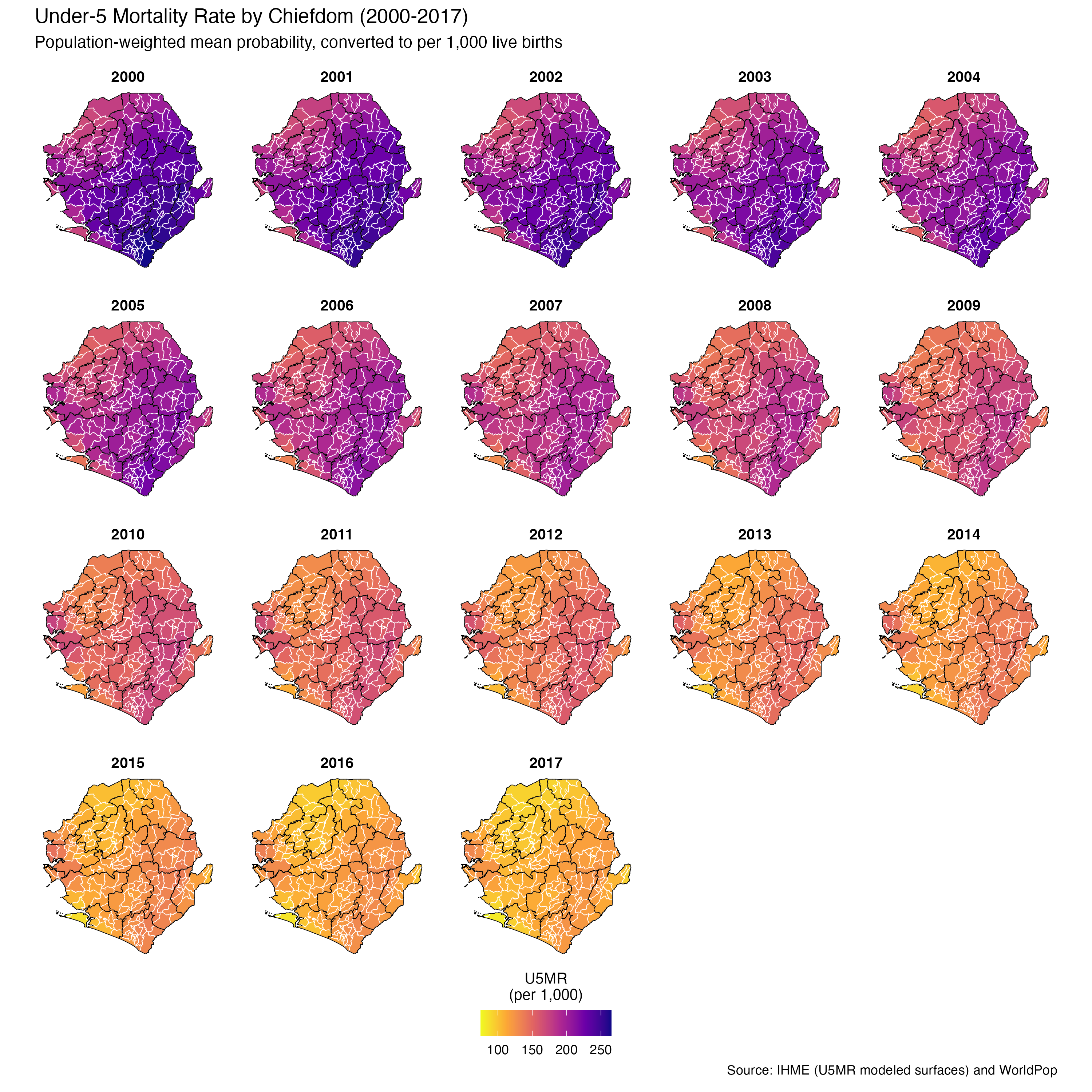
ggplot2::labs(
title = "Under-5 Mortality Rate by Chiefdom (2000-2017)",
subtitle = paste0(
"Population-weighted mean probability, ",
"converted to per 1,000 live births\n"
),
caption = "Source: IHME (U5MR modeled surfaces) and WorldPop\n"
) +
ggplot2::theme_void() +
ggplot2::theme(
legend.position = "bottom",
legend.title = ggplot2::element_text(size = 10),
strip.text = ggplot2::element_text(face = "bold", size = 10),
panel.spacing = ggplot2::unit(1, "lines")
)
u5mr_map_weighted
NoteOutput
To adapt the code:
- Line 14: Ensure
u5mr_mean_weightedis the correct column name from your final data - Line 46: Adjust
facet_wrap(~ year)to another level if preferred. - If you would like to use a binned version for plotting, please refer to Step 3.2, in particular lines 810-816 for the binning of u5mr_mean_weighted, and lines 838-846 for the setup of fill colours.
- Lines 47–50: Update titles or captions as needed.
Once updated, run the code to generate the plot.
Python
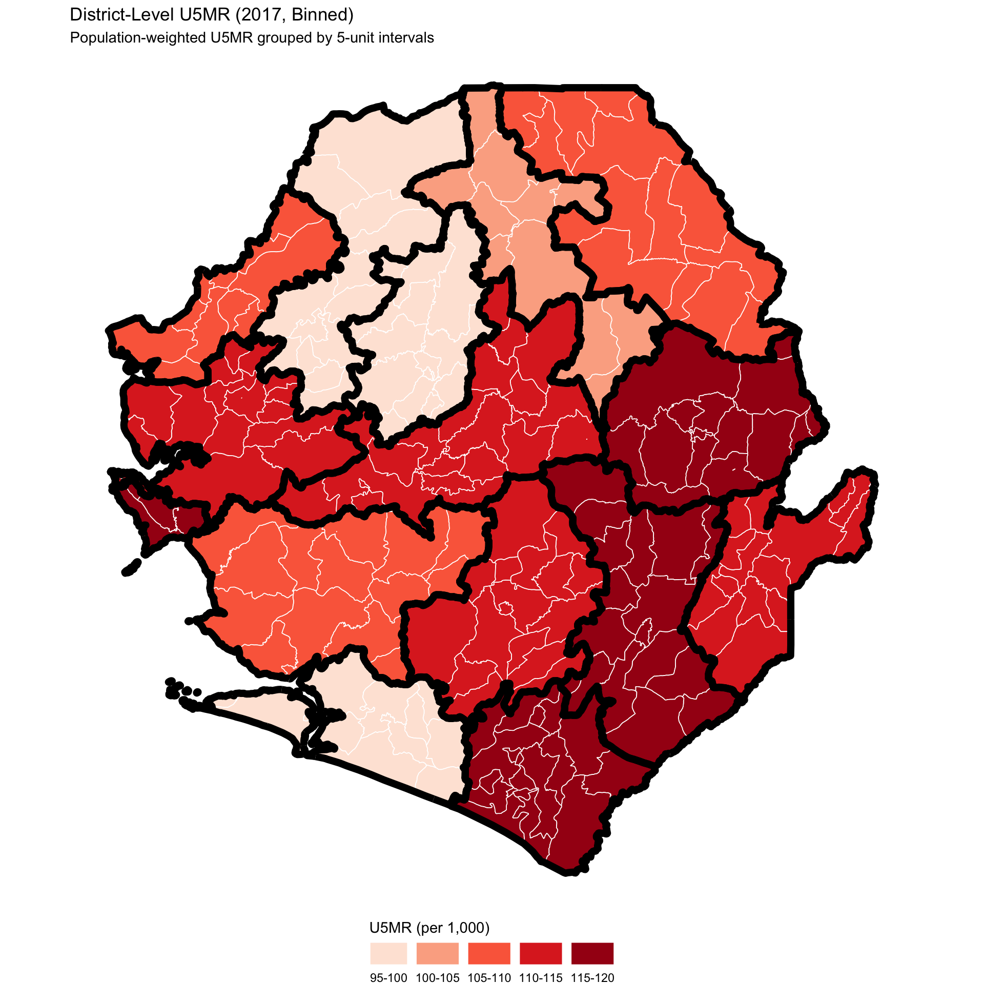
Step 3.2: Focusing on 2017 - single-year U5MR map
Focusing on 2017, we map district-level (adm2) U5MR to highlight spatial variation. U5MR values in 2017 range from 96.6 to 120.2 per 1,000 live births, so we bin them into 5-unit intervals to improve readability and facilitate district-level comparisons. To enhance visual clarity, we also apply a diverging red color scheme to highlight relative differences across bins.
ImportantConsult SNT Team
Thresholds used to classify continuous indicators should be discussed with the SNT team. Include plots and summary tables in outputs to support transparent and reproducible threshold decisions, visualize indicator distributions over time, and show how many districts fall into each threshold category. This helps assess the operational implications.
Remember, a single indicator may need different thresholds for different purposes (e.g., lower thresholds for elimination, higher for campaign planning). These decisions should be made by the SNT team.
Show full code
# Filter for 2017 and aggregate to adm2
u5mr_2017_adm2 <- u5mr_final_shp |>
dplyr::filter(year == 2017) |>
dplyr::mutate(u5mr_per1000 = u5mr_mean_weighted * 1000) |>
dplyr::group_by(adm0, adm1, adm2) |>
dplyr::summarise(
u5mr_per1000 = base::mean(u5mr_per1000, na.rm = TRUE),
.groups = "drop"
) |>
dplyr::mutate(
u5mr_bin = base::cut(
u5mr_per1000,
breaks = c(95, 100, 105, 110, 115, 120.5),
labels = c("95-100", "100-105", "105-110", "110-115", "115-120"),
include.lowest = TRUE
)
) |>
dplyr::left_join(
sle_shp |> dplyr::select(adm0, adm1, adm2),
by = c("adm0", "adm1", "adm2")
) |>
sf::st_as_sf()
# Plot with custom theme
p <- ggplot2::ggplot(u5mr_2017_adm2) +
ggplot2::geom_sf(
ggplot2::aes(fill = u5mr_bin),
color = NA,
size = 0.3
) +
# Add adm1 outline as a black border
ggplot2::geom_sf(
data = shp_adm2,
fill = NA,
color = "black",
size = 2.5
) +
ggplot2::scale_fill_manual(
name = "U5MR (per 1,000)",
values = c(
"95-100" = "#fee5d9",
"100-105" = "#fcae91",
"105-110" = "#fb6a4a",
"110-115" = "#de2d26",
"115-120" = "#a50f15"
),
na.value = "grey80",
guide = ggplot2::guide_legend(
label.position = "bottom",
title.position = "top"
)
) +
ggplot2::labs(
title = "District-Level U5MR (2017, Binned)",
subtitle = "Population-weighted U5MR grouped by 5-unit intervals"
) +
ggplot2::theme_void() +
ggplot2::theme(
legend.position = "bottom",
legend.title.position = "top",
legend.key.width = grid::unit(1, "cm")
)
p
NoteOutput
To adapt the code:
- Line 10: Ensure
u5mr_mean_weightedis the correct column name for your 2017 U5MR values. - Lines 11–12: Confirm that
adm2refers to your district-level administrative unit. - Lines 17–21: Adjust the
cut()breakpoints or labels if your value range differs. - Lines 59–61: Update map titles or subtitles to reflect your context.
Once updated, run the code to generate the district-level map for 2017.
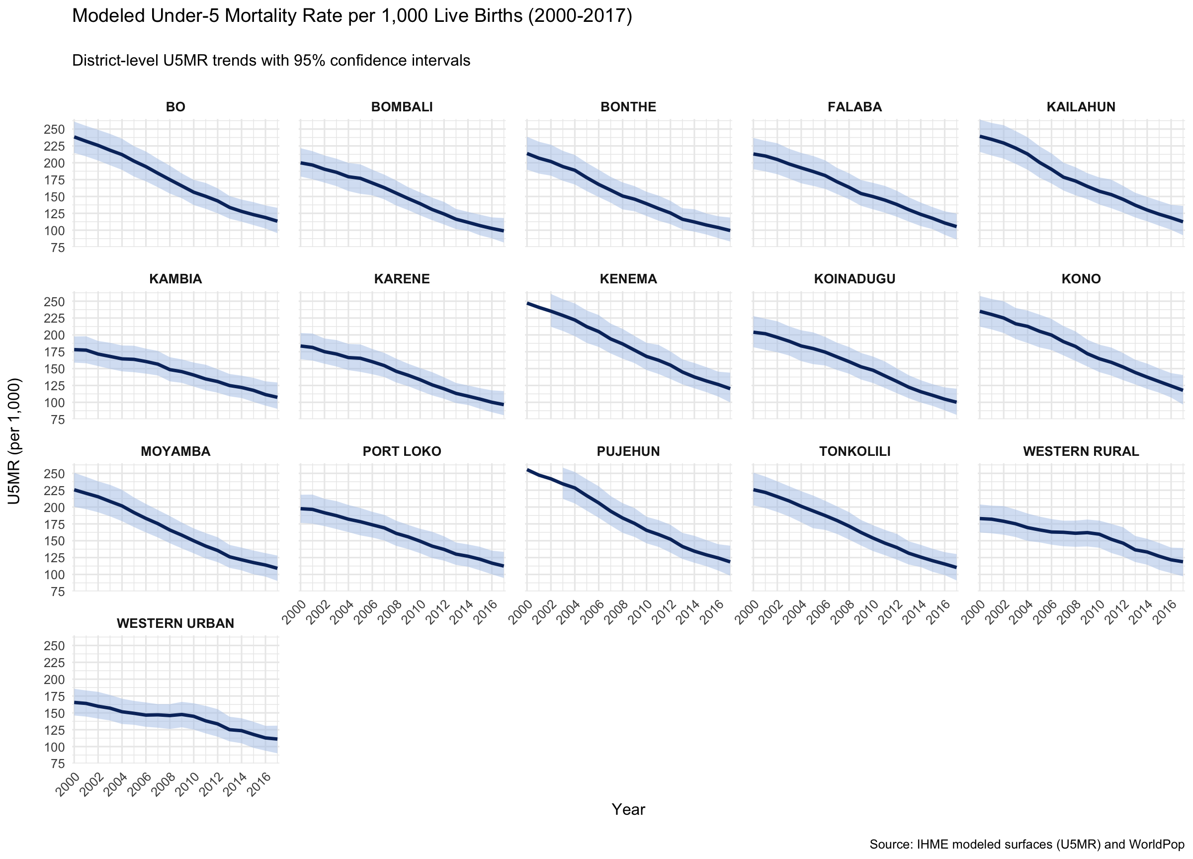
Step 3.3: Visualize U5MR trends
In this step, we visualize annual trends in U5MR across all Chiefdom from 2000 to 2017. The maps show the population-weighted mean U5MR, while also incorporating confidence intervals to reflect uncertainty in the modeled estimates.
Show full code
u5mr_trend <- u5mr_final_shp |>
dplyr::mutate(
u5mr_per1000 = u5mr_mean_weighted * 1000,
u5mr_lower_per1000 = u5mr_lower_weighted * 1000,
u5mr_upper_per1000 = u5mr_upper_weighted * 1000
) |>
dplyr::group_by(adm0, adm1, adm2, year) |>
dplyr::summarise(
u5mr_per1000 = base::mean(u5mr_per1000, na.rm = TRUE),
u5mr_lower_per1000 = base::mean(u5mr_lower_per1000, na.rm = TRUE),
u5mr_upper_per1000 = base::mean(u5mr_upper_per1000, na.rm = TRUE),
.groups = "drop"
) |>
ggplot2::ggplot(ggplot2::aes(x = year)) +
ggplot2::geom_ribbon(
ggplot2::aes(
ymin = u5mr_lower_per1000,
ymax = u5mr_upper_per1000
),
fill = "#aec7e8",
alpha = 0.5
) +
ggplot2::geom_line(
ggplot2::aes(y = u5mr_per1000),
color = "#08306B",
size = 1.2
) +
ggplot2::scale_x_continuous(
limits = c(2000, 2017),
breaks = base::seq(2000, 2017, 2),
expand = c(0.01, 0)
) +
ggplot2::scale_y_continuous(
limits = c(75, 265),
breaks = base::seq(75, 265, 25),
expand = c(0, 0)
) +
ggplot2::facet_wrap(~adm2, ncol = 5) +
ggplot2::labs(
title = paste0(
"Modeled Under-5 Mortality Rate ",
"per 1,000 Live Births (2000-2017)\n"
),
subtitle = "District-level U5MR trends with 95% confidence intervals\n",
y = "U5MR (per 1,000)\n",
x = "Year",
caption = "\nSource: IHME modeled surfaces (U5MR) and WorldPop"
) +
ggplot2::theme_minimal(base_size = 12) +
ggplot2::theme(
strip.text = ggplot2::element_text(face = "bold", size = 10),
axis.text.x = ggplot2::element_text(angle = 45, hjust = 1),
panel.spacing = ggplot2::unit(1, "lines"),
legend.position = "none"
)
u5mr_trend
NoteOutput
To adapt the code:
- Lines 11–13: Ensure
u5mr_mean_weighted,u5mr_lower_weighted, andu5mr_upper_weightedare the correct column names from your aggregation step. - Line 46: Adjust
facet_wrap(~ adm2)to another level (e.g.,adm1) if preferred. - Lines 47–52: Update titles or captions as needed.
Once updated, run the code to generate the plot.
ImportantValidate Results with SNT Team
Before finalizing IHME-modeled U5MR outputs, analysts should review categorized maps alongside known benchmarks to validate their alignment with local expectations.
A useful check is to compare the binned U5MR map for the DHS survey year to direct DHS-based mortality estimates (see DHS Mortality section). This provides a second line of evidence and helps ground the modeled outputs in observed data.
Key questions for review with the SNT team:
- Do the spatial patterns match what is known from programmatic experience?
- Are there areas where the model results conflict with DHS estimates?
- Are any trends unexpected or needing clarification?
Include both the IHME and DHS-based maps in the output package to support a structured validation discussion.
Step 4: Save Processed U5MR Estimates and Plots
We now save the processed U5MR outputs and their associated visualizations. These include the weighted Chiefdom-level summaries across time as well as the multi-year faceted map.
# Save faceted map of weighted U5MR with WHO groupings
ggplot2::ggsave(
plot = u5mr_map_weighted,
here::here(
"03_output/3a_figures/u5mr_map_weighted_adm2_2000_2017.png"
),
width = 12,
height = 7,
dpi = 300
)
# Save U5MR temporal trend plot if available
ggplot2::ggsave(
plot = u5mr_trend,
here::here(
"03_output/3a_figures/u5mr_trend_adm2_2000_2017.png"
),
width = 12,
height = 7,
dpi = 300
)
# Define save path
save_path <- here::here("1.2_epidemiology/1.2c_mortality_estimates")
# Save processed data as CSV
rio::export(
u5mr_final,
here::here(
save_path, "processed", "u5mr_processed_adm2_2000_2017.csv"
)
)
# Save processed data as RDS
rio::export(
u5mr_final,
here::here(
save_path, "processed", "final_u5mr_processed_adm2_2000_2017.rds"
)
)To adapt the code:
- Lines 3, 12: Replace u5mr_map_weighted and u5mr_trend with your actual ggplot object names.
- Lines 4–6, 13–15, 25–27, 32–34: Adjust file names and locations as needed to reflect your naming conventions and output directory.
- Lines 26, 32: Update
u5mr_finalto match your final dataset name and edit file names accordingly (e.g., if using a different admin level or time span).
Once updated, run the code to store your mortality estimates and figures for further use, validation, or publication.
Summary
This section guided you through saving processed U5MR estimates and related plots. The outputs reflect Chiefdom-level, population-weighted summaries, enabling interpretation of both spatial patterns and temporal changes in child mortality. These files are now ready for use in reporting, further stratification, or integration into broader SNT workflows.
Full code
Find the full code script for accessing and processing IHME mortality estimates below.
Show full code
################################################################################
####### ~ Modeled estimates of malaria mortality and proxies full code ~ #######
################################################################################
### Step 1: Initial Setup, Check and Load IHME Rasters -------------------------
#### Step 1.1: Initial setup ---------------------------------------------------
# Load required packages
pacman::p_load(
terra, # For raster operations
sf, # For vector data
dplyr, # For data manipulation
here, # For file path management
glue # For dynamic string construction
)
# Download latest sntutils if you haven't already
devtools::install_github("ahadi-analytics/sntutils")
# Define folder to store IHME surfaces
maps_data_path <- here::here(
"1.2_epidemiology/1.2c_mortality_estimates/raw"
)
# Load admin boundary shapefile
sle_shp <- readRDS(
here::here(
"1.1_foundational/1a_admin_boundaries",
"1ai_adm3",
"sle_spatial_adm3_2021.rds"
)
)
#### Step 1.3 Import rasters ---------------------------------------------------
# Get the mean U5MR
stacked_rast_u5mr_mean <- terra::rast(
here::here(maps_data_path,
"IHME_LMICS_U5M_2000_2017_Q_UNDER5_MEAN_Y2019M10D16.TIF")
)
# Get the upper bound U5MR
stacked_rast_u5mr_upper <- terra::rast(
here::here(maps_data_path,
"IHME_LMICS_U5M_2000_2017_Q_UNDER5_UPPER_Y2019M10D16.TIF")
)
# Get the lower bound U5MR
stacked_rast_u5mr_lower <- terra::rast(
here::here(maps_data_path,
"IHME_LMICS_U5M_2000_2017_Q_UNDER5_LOWER_Y2019M10D16.TIF")
)
#### Step 1.4 Selecting rasters ------------------------------------------------
# Example: extract 2010-2017 period
years_to_use <- 11:18

rast_u5mr_mean   <- stacked_rast_u5mr_mean[[years_to_use]]
rast_u5mr_upper  <- stacked_rast_u5mr_upper[[years_to_use]]
rast_u5mr_lower  <- stacked_rast_u5mr_lower[[years_to_use]]
# Select full 2000-2017 range (default)
rast_u5mr_mean  <- stacked_rast_u5mr_mean
rast_u5mr_upper <- stacked_rast_u5mr_upper
rast_u5mr_lower <- stacked_rast_u5mr_lower
### Step 2: Extract and Aggregate U5MR from IHME Rasters to Administrative Units
#### Step 2.1: Aggregate population-weighted U5MR (Option A, recommended method)
# Set up output path
worldpop_rast_path <- here::here(
  "01_data",
  "1.1_foundational",
  "1.1c_population",
  "1.1ci_worldpop_rasters"
)

# Download pop data
sntutils::download_worldpop(
  country_codes = "SLE",
  years = 2000:2017,
  dest_dir = here::here(worldpop_rast_path, "raw"),
)
# List all WorldPop raster files
raster_files <- base::list.files(
  path = here::here(worldpop_rast_path, "raw"),
  pattern = "\\.tif$",
  full.names = TRUE
)

# Combine into one raster stack
pop_wp_raster_stack <- terra::rast(raster_files[1:18])

# Extract the weighted U5MR mean estimate
u5mr_mean_df <- sntutils::process_weighted_raster_stacks(
  value_raster = rast_u5mr_mean,
  pop_raster = pop_wp_raster_stack,
  shape = sle_shp,
  value_var = "u5mr_mean_weighted",
  stat_type = "mean"
)

# Extract the weighted U5MR lower estimate
u5mr_lower_df <- sntutils::process_weighted_raster_stacks(
  value_raster = rast_u5mr_lower,
  pop_raster = pop_wp_raster_stack,
  shape = sle_shp,
  value_var = "u5mr_lower_weighted",
  stat_type = "mean"
)

# Extract the weighted U5MR upper estimate
u5mr_upper_df <- sntutils::process_weighted_raster_stacks(
  value_raster = rast_u5mr_upper,
  pop_raster = pop_wp_raster_stack,
  shape = sle_shp,
  value_var = "u5mr_upper_weighted",
  stat_type = "mean"
)

# Now join all U5MR outputs into one
u5mr_final <- u5mr_mean_df |>
  dplyr::left_join(
    u5mr_lower_df,
    by = c("adm0", "adm1", "adm2", "adm3", "geometry_hash", "year"),
  ) |>
  dplyr::left_join(
    u5mr_upper_df,
    by = c("adm0", "adm1", "adm2", "adm3", "geometry_hash", "year"),
  )

# Check the final output
u5mr_final |>
  dplyr::select(-adm0, -geometry_hash) |>
  utils::head()
#### Step 2.2: Aggregate unweighted U5MR (Option B) ----------------------------
# Extract mean mortality counts (central estimates) for all years
ihme_mean <- sntutils::process_ihme_u5m_raster(
  shape = sle_shp,
  raster_stack = rast_u5mr_mean,
  id_col = c("adm0", "adm1", "adm2", "adm3", "geometry_hash"),
  stat_type = "mean"
) |>
  dplyr::rename(u5mr_mean = u5m_rate)

# Extract lower bound estimates
ihme_lower <- sntutils::process_ihme_u5m_raster(
  shape = sle_shp,
  raster_stack = rast_u5mr_lower,
  id_col = "geometry_hash",
  stat_type = "mean"
) |>
  dplyr::rename(u5mr_lower = u5m_rate)

# Extract upper bound estimates
ihme_upper <- sntutils::process_ihme_u5m_raster(
  shape = sle_shp,
  raster_stack = rast_u5mr_upper,
  id_col = "geometry_hash",
  stat_type = "mean"
) |>
  dplyr::rename(u5mr_upper = u5m_rate)

# Join all three together by geometry_hash and year
u5mr_final_unweighted <- ihme_mean |>
  dplyr::left_join(ihme_lower, by = c("geometry_hash", "year")) |>
  dplyr::left_join(ihme_upper, by = c("geometry_hash", "year"))

# Check unweighted output
u5mr_final_unweighted |>
  dplyr::select(-adm0, -geometry_hash) |>
  utils::head()
### Step 3: Visualize U5MR Spatial Distribution and Temporal Trends ------------
#### Step 3.1: Visualize U5MR spatial distribution -----------------------------
# Generate adm1-level shapefile
shp_adm1 <- sle_shp |>
  sf::st_as_sf() |>
  dplyr::group_by(adm1) |>
  dplyr::summarise(geometry = sf::st_union(geometry), .groups = "drop")

# Generate adm2-level shapefile
shp_adm2 <- sle_shp |>
  sf::st_as_sf() |>
  dplyr::group_by(adm2) |>
  dplyr::summarise(geometry = sf::st_union(geometry), .groups = "drop")

# Map U5MR trends over space and time
u5mr_final_shp <- u5mr_final |>
  dplyr::left_join(
    sle_shp |> dplyr::select(geometry_hash),
    by = "geometry_hash"
  )

u5mr_map_unweighted <- u5mr_final_shp |>
  sf::st_as_sf() |>
  ggplot2::ggplot() +
  ggplot2::geom_sf(
    ggplot2::aes(fill = u5mr_mean),
    color = "white",
    size = 0.2
  ) +
  # Add adm1 outline as a black border
  ggplot2::geom_sf(
    data = shp_adm2,
    fill = NA,
    color = "black",
    size = 2.5
  ) +
  ggplot2::scale_fill_viridis_c(
    option = "C",
    direction = -1,
    name = "U5MR\n(per 1,000)",
    labels = scales::number_format(scale = 1000, accuracy = 1),
    limits = c(0.075, 0.265),
    na.value = "transparent",
    oob = scales::squish,
    guide = ggplot2::guide_colorbar(
      label.position = "bottom",
      title.position = "top",
      title.hjust = 0.5,
      override.aes = list(
        colour = "black",
        size = 0.15,
        alpha = 1
      ),
      nrow = 1,
      byrow = TRUE
    )
  ) +
  ggplot2::facet_wrap(~year, ncol = 5) +
  ggplot2::labs(
    title = "Under-5 Mortality Rate by Chiefdom (2000-2017)",
    subtitle = paste0(
      "Unweighted mean probability, ",
      "converted to per 1,000 live births\n"
    ),
    caption = "Source: IHME (U5MR modeled surfaces)\n"
  ) +
  ggplot2::theme_void() +
  ggplot2::theme(
    legend.position = "bottom",
    legend.title = ggplot2::element_text(size = 10),
    strip.text = ggplot2::element_text(face = "bold", size = 10),
    panel.spacing = ggplot2::unit(1, "lines")
  )

u5mr_map_unweighted
# Map unweighted U5MR
u5mr_map_weighted <- u5mr_final_shp |>
  sf::st_as_sf() |>
  ggplot2::ggplot() +
  ggplot2::geom_sf(
    ggplot2::aes(fill = u5mr_mean_weighted),
    color = "white",
    size = 0.2
  ) +
  # Add adm1 outline as a black border
  ggplot2::geom_sf(
    data = shp_adm2,
    fill = NA,
    color = "black",
    size = 2.5
  ) +
  ggplot2::scale_fill_viridis_c(
    option = "C",
    direction = -1,
    name = "U5MR\n(per 1,000)",
    labels = scales::number_format(scale = 1000, accuracy = 1),
    limits = c(0.075, 0.265),
    na.value = "transparent",
    oob = scales::squish,
    guide = ggplot2::guide_colorbar(
      label.position = "bottom",
      title.position = "top",
      title.hjust = 0.5,
      override.aes = list(
        colour = "black",
        size = 0.15,
        alpha = 1
      ),
      nrow = 1,
      byrow = TRUE
    )
  ) +
  ggplot2::facet_wrap(~year, ncol = 5) +
  ggplot2::labs(
    title = "Under-5 Mortality Rate by Chiefdom (2000-2017)",
    subtitle = paste0(
      "Population-weighted mean probability, ",
      "converted to per 1,000 live births\n"
    ),
    caption = "Source: IHME (U5MR modeled surfaces) and WorldPop\n"
  ) +
  ggplot2::theme_void() +
  ggplot2::theme(
    legend.position = "bottom",
    legend.title = ggplot2::element_text(size = 10),
    strip.text = ggplot2::element_text(face = "bold", size = 10),
    panel.spacing = ggplot2::unit(1, "lines")
  )

u5mr_map_weighted
#### Step 3.2: Focusing on 2017 - single-year U5MR map -------------------------
# Filter for 2017 and aggregate to adm2
u5mr_2017_adm2 <- u5mr_final_shp |>
  dplyr::filter(year == 2017) |>
  dplyr::mutate(u5mr_per1000 = u5mr_mean_weighted * 1000) |>
  dplyr::group_by(adm0, adm1, adm2) |>
  dplyr::summarise(
    u5mr_per1000 = base::mean(u5mr_per1000, na.rm = TRUE),
    .groups = "drop"
  ) |>
  dplyr::mutate(
    u5mr_bin = base::cut(
      u5mr_per1000,
      breaks = c(95, 100, 105, 110, 115, 120.5),
      labels = c("95-100", "100-105", "105-110", "110-115", "115-120"),
      include.lowest = TRUE
    )
  ) |>
  dplyr::left_join(
    sle_shp |> dplyr::select(adm0, adm1, adm2),
    by = c("adm0", "adm1", "adm2")
  ) |>
  sf::st_as_sf()

# Plot with custom theme
p <- ggplot2::ggplot(u5mr_2017_adm2) +
  ggplot2::geom_sf(
    ggplot2::aes(fill = u5mr_bin),
    color = NA,
    size = 0.3
  ) +
  # Add adm1 outline as a black border
  ggplot2::geom_sf(
    data = shp_adm2,
    fill = NA,
    color = "black",
    size = 2.5
  ) +
  ggplot2::scale_fill_manual(
    name = "U5MR (per 1,000)",
    values = c(
      "95-100" = "#fee5d9",
      "100-105" = "#fcae91",
      "105-110" = "#fb6a4a",
      "110-115" = "#de2d26",
      "115-120" = "#a50f15"
    ),
    na.value = "grey80",
    guide = ggplot2::guide_legend(
      label.position = "bottom",
      title.position = "top"
    )
  ) +
  ggplot2::labs(
    title = "District-Level U5MR (2017, Binned)",
    subtitle = "Population-weighted U5MR grouped by 5-unit intervals"
  ) +
  ggplot2::theme_void() +
  ggplot2::theme(
    legend.position = "bottom",
    legend.title.position = "top",
    legend.key.width = grid::unit(1, "cm")
  )

p
#### Step 3.3: Visualize U5MR trends -------------------------------------------
u5mr_trend <- u5mr_final_shp |>
  dplyr::mutate(
    u5mr_per1000 = u5mr_mean_weighted * 1000,
    u5mr_lower_per1000 = u5mr_lower_weighted * 1000,
    u5mr_upper_per1000 = u5mr_upper_weighted * 1000
  ) |>
  dplyr::group_by(adm0, adm1, adm2, year) |>
  dplyr::summarise(
    u5mr_per1000 = base::mean(u5mr_per1000, na.rm = TRUE),
    u5mr_lower_per1000 = base::mean(u5mr_lower_per1000, na.rm = TRUE),
    u5mr_upper_per1000 = base::mean(u5mr_upper_per1000, na.rm = TRUE),
    .groups = "drop"
  ) |>
  ggplot2::ggplot(ggplot2::aes(x = year)) +
  ggplot2::geom_ribbon(
    ggplot2::aes(
      ymin = u5mr_lower_per1000,
      ymax = u5mr_upper_per1000
    ),
    fill = "#aec7e8",
    alpha = 0.5
  ) +
  ggplot2::geom_line(
    ggplot2::aes(y = u5mr_per1000),
    color = "#08306B",
    size = 1.2
  ) +
  ggplot2::scale_x_continuous(
    limits = c(2000, 2017),
    breaks = base::seq(2000, 2017, 2),
    expand = c(0.01, 0)
  ) +
  ggplot2::scale_y_continuous(
    limits = c(75, 265),
    breaks = base::seq(75, 265, 25),
    expand = c(0, 0)
  ) +
  ggplot2::facet_wrap(~adm2, ncol = 5) +
  ggplot2::labs(
    title = paste0(
      "Modeled Under-5 Mortality Rate ",
      "per 1,000 Live Births (2000-2017)\n"
    ),
    subtitle = "District-level U5MR trends with 95% confidence intervals\n",
    y = "U5MR (per 1,000)\n",
    x = "Year",
    caption = "\nSource: IHME modeled surfaces (U5MR) and WorldPop"
  ) +
  ggplot2::theme_minimal(base_size = 12) +
  ggplot2::theme(
    strip.text = ggplot2::element_text(face = "bold", size = 10),
    axis.text.x = ggplot2::element_text(angle = 45, hjust = 1),
    panel.spacing = ggplot2::unit(1, "lines"),
    legend.position = "none"
  )

u5mr_trend
### Step 4: Save Processed U5MR Estimates and Plots ----------------------------
# Save faceted map of weighted U5MR with WHO groupings
ggplot2::ggsave(
  plot = u5mr_map_weighted,
  here::here(
    "03_output/3a_figures/u5mr_map_weighted_adm2_2000_2017.png"
  ),
  width = 12,
  height = 7,
  dpi = 300
)

# Save U5MR temporal trend plot if available
ggplot2::ggsave(
  plot = u5mr_trend,
  here::here(
    "03_output/3a_figures/u5mr_trend_adm2_2000_2017.png"
  ),
  width = 12,
  height = 7,
  dpi = 300
)

# Define save path
save_path <- here::here("1.2_epidemiology/1.2c_mortality_estimates")

# Save processed data as CSV
rio::export(
  u5mr_final,
  here::here(
    save_path, "processed", "u5mr_processed_adm2_2000_2017.csv"
  )
)

# Save processed data as RDS
rio::export(
  u5mr_final,
  here::here(
    save_path, "processed", "final_u5mr_processed_adm2_2000_2017.rds"
  )
)