# load required packages
pacman::p_load(
  terra,       # for raster operations
  sf,          # for vector data
  exactextractr, # for precise extraction from rasters
  dplyr,       # for data manipulation
  lubridate,   # for date handling
  here        # for file path management
)

# download latest sntutils if you haven't already
devtools::install_github("ahadi-analytics/sntutils")

# import administrative boundary shapefile
sl_adm3_shp <- readRDS(
  here::here("01_foundational/1a_administrative_boundaries",
             "1ai_adm3", "sle_spatial_adm3_2021.rds")
) |> sf::st_as_sf() # ensure it gets turned into sf formatClimate and environment data extraction from raster
Overview
Environmental conditions, particularly rainfall, temperature, vegetation, and proximity to water, play a fundamental role in shaping malaria transmission. They influence both the habitats where mosquitoes breed and the biological processes that govern transmission. Variables such as rainfall, temperature, and humidity affect mosquito survival, breeding site availability, and the rate at which parasites develop within the vector. These factors often vary seasonally and geographically, making their analysis highly informative for SNT.
As part of the SNT process, climate data is incorporated early during data assembly to ensure environmental conditions are appropriately reflected in downstream analyses. Cleaned, monthly summaries of key climate variables are aggregated to the operational unit for analysis (typically adm2 or adm3 level) to support stratification of determinants of malaria transmission.
NoteObjectives
- Identify suitable climate data sources for SNT
- Understand how CHIRPS raster files are structured and accessed
- Download and preview monthly rainfall rasters from CHIRPS
- Extract rainfall summaries per subnational level using shapefiles
- Batch process multiple rasters and prepare data for SNT workflows
Types of Climate and Environment Data Available
With the growing availability of remote sensing and other big-data sources, teams now have access to an expanding set of climate products, each with trade-offs in coverage, resolution, accessibility, and validation. There is no single correct dataset for SNT. The examples below reflect widely used, open-access sources, but countries may choose different datasets based on availability, spatial or temporal detail, infrastructure available, or endorsement by national programs.
ImportantConsult SNT Team
Always start by asking the SNT team if they have data from their own meteorological or weather stations. Even if weather stations are not everywhere, they can serve as a very reliable source of information to confirm that the data extracted from satellite imagery or other sources is capturing what happened in reality.
| Source | Type | Format | Resolution | Access & Notes |
|---|---|---|---|---|
| CHIRPS | Rainfall | Daily, monthly | ~5km | Available via web UI or programmatically using the chirps R package. Ideal for subnational summaries. |
| MODIS NDVI | Vegetation index | 16-day composite | 250m | NDVI rasters available via MODIS NDVI product page (MOD13Q1). Often used to monitor seasonal vegetation dynamics and land cover conditions. |
| AVHRR NDVI | Vegetation index | 16-day composite | ~4 km | Long-term record since the 1980s. Available via NOAA’s archive. |
| IMERG | Rainfall | Half-hourly, daily | ~10km | Satellite-based global precipitation estimates from NASA GPM. Useful for near-real-time monitoring. Accessible via NASA GES DISC. Requires preprocessing for analysis. |
| WorldClim | Climate normals | Monthly, derived | ~1km | Historical climate averages (baseline period). Useful for deriving suitability or comparing anomalies. |
| CRU TS | Climate trend data | Monthly | ~50km | Covers 1901–present. Widely used in academic modeling; coarse spatial detail. |
| National Met Offices* | Gauge or grid | Varies | Varies | Often the gold standard for programmatic use if available. Access may require a formal request, typically coordinated by the SNT team. Example: Sierra Leone National Water Resources Management Agency provides local rainfall summaries by request. |
Note: National Met Offices* provide direct observational data, not model-derived estimates like the others.
Each dataset involves trade-offs across temporal coverage, spatial resolution, usability, and processing burden. The best choice depends on the intended analysis and your team’s operational setup. Consider:
Time period: Do you need near-real-time observations (e.g., for early warning), or long-term historical data (e.g., for climatological baselines)? Some datasets offer daily records from the 1980s onward; others provide only monthly summaries or static climate normals. For most SNT workflows, monthly resolution is the minimum granularity required. Daily data can always be aggregated up to monthly values.
Spatial resolution: Are you working at the district (adm2/adm3) level, or is a coarser scale sufficient? CHIRPS provides ~5 km resolution suitable for subnational summaries. Others, like ERA5 or IMERG, can offer finer resolution (1 km or better), but this increases complexity and file size. Finer resolution doesn’t always imply better accuracy, particularly in areas with sparse ground validation.
Infrastructure requirements: High-resolution datasets (e.g., daily at 10 m) can be demanding in terms of storage, bandwidth, and computing. Multi-year downloads may involve gigabytes of data, and processing may exceed standard laptop capacity. For many workflows, coarser rasters or pre-aggregated tables are more practical. Assess whether your infrastructure can handle large raster workflows, or if a simplified approach is preferable.
Country preference: Some countries have preferred sources, such as national meteorological agencies or approved datasets. Where these are accessible and endorsed, they may offer programmatic advantages. However, access is often restricted and these sources may not always be available in formats or timelines that meet the operational needs of SNT analysis.
TipNot sure what to use?
What is presented here is not prescriptive. The goal is fit-for-purpose climate indicators that match your operational needs. If in doubt, consult with national counterparts or the SNT team to confirm appropriate data sources and formats.
Choosing between these different datasets depends on context. For example:
If your goal is to extract rainfall data from 2020 to 2023 at the adm3 level, you’ll need a dataset that provides continuous coverage over those years, with sufficient spatial resolution to reflect subnational variation. In such cases, open-source gridded datasets like CHIRPS (for rainfall) or ERA5 (for temperature) are good candidates.
These datasets are updated regularly, cover most malaria-endemic countries, and allow for either pixel-level raster extraction or coordinate-based querying depending on your workflow. Their moderate resolution (typically between 5 km and 30 km) makes them efficient to download, store, and process: monthly summaries can be handled on standard laptops without requiring high-performance computing.
In this section, we demonstrate how to work with full-resolution climate rasters (e.g., CHIRPS .tif files) for teams that rely on this dataset or already have bulk raster data available. While the examples use CHIRPS, the same workflow can be adapted for other gridded raster datasets with similar structure. Note that working with national meteorological data, when provided in summary tables or other non-raster formats, is not covered here.
Step-by-Step
Step 1: Set-up and Download CHIRPS Raster Files
The first step is to download CHIRPS raster files for our area of interest. While these can be obtained manually from the CHIRPS website, we use a custom function from the sntutils package to automate this process for Africa. Before doing so, we install the required packages, load the necessary functions, and import the shapefile for later spatial extraction.
To skip the step-by-step explanation, jump to the full code at the end of this page.
Step 1.1: Initial set-up
To adapt the code:
- Lines 15–17: Update the file path to match where your administrative boundary shapefile is stored (e.g.,
your/path/to/shapefile.rds). - Line 17: Change
"sle_spatial_adm3_2021.rds"to match your actual shapefile name.
Once updated, run the code to load your administrative boundary shapefile.
If you already have CHIRPS .tif files downloaded, or prefer to manage downloads manually without using sntutils, you can skip Step 1.3 and go straight to Step 2.
Step 1.2: Check available CHIRPS datasets
Before downloading any data, it’s a good idea to inspect which CHIRPS datasets are supported. The chirps_options() function from sntutils returns a tidy list of available datasets, including their region and time aggregation (e.g., monthly).
After identifying a dataset of interest (e.g., africa_monthly), you can check the available years and months for download using check_chirps_available().
It appears data is available from January 1981 to March 2025, covering all months in this period up to the latest available release.
Step 1.3: Download CHIRPS raster data
Now that we’ve confirmed data availability, we proceed to download 48 monthly CHIRPS rainfall rasters for Africa, covering January 2020 to December 2023. Each file captures total rainfall in millimetres across the continent at ~5km resolution. The download_chirps() function handles the download and optional unzipping, saving files with clear dataset-prefixed names to the specified directory. This setup can be easily modified for other regions or time periods using available options from chirps_options().
To adapt the code:
- Line 2: Change
"05_climate_and environment"to the working directory where you want to store your climate data. - Line 5: Specify your dataset of interest, based on your region and available options in
chirps_options(). - Lines 6–7: Define the start and end dates for your desired time period.
Once updated, run the code to fully download your CHIRPS data.
In this example focusing on Africa, each compressed file is roughly 5 MB, so downloading all 48 should take no more than 15 minutes with a reasonable internet connection.
Step 2: Load, Inspect, and Process a Single CHIRPS Raster
Before we scale up to process all CHIRPS rasters, it’s useful to walk through the steps for a single .tif file, to understand how the data is handled and transformed. We’ll use the May 2023 raster file as an example.
If you prefer to skip this detailed step-by-step illustration and go straight to processing all rasters at once, you can jump to Step 3 below. Otherwise, follow along to understand how the batch function works under the hood.
Step 2.1: Load and clean the raster
We read in the raster, convert CHIRPS missing values (coded as -9999) to NA, and preview the file.
Step 2.2: Visualize the raster
Now we visualise the raster to check that it is correctly loaded and represents realistic spatial patterns.
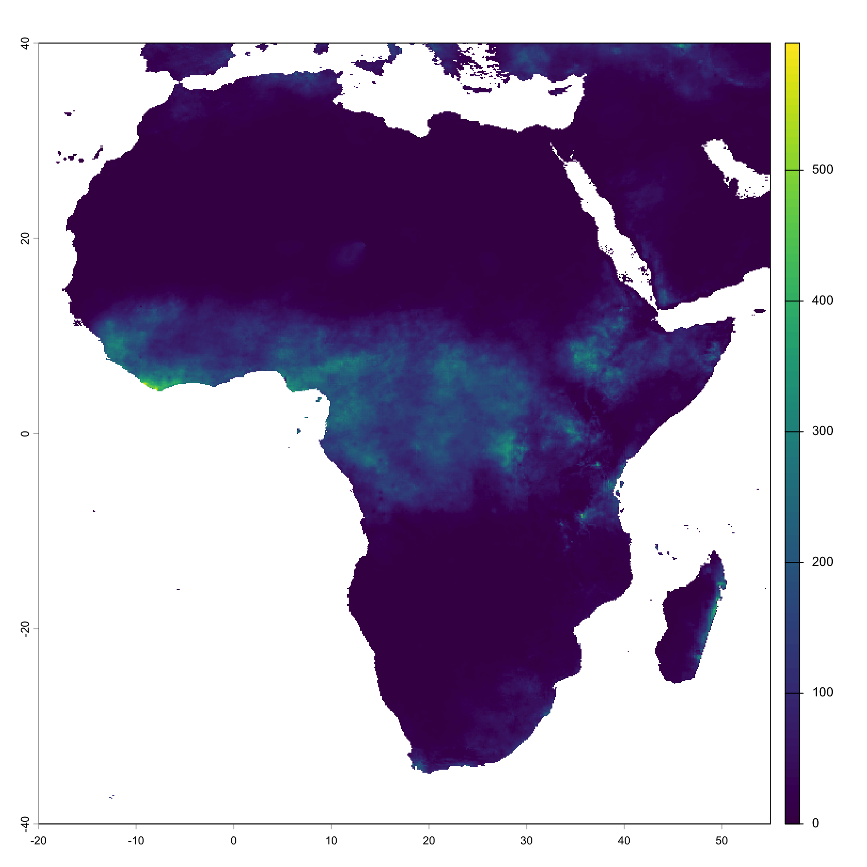
With the raster loaded and visualized, we see rainfall distribution across Africa for May 2023. High rainfall in Central and West Africa aligns with expected seasonal patterns. This confirms the CHIRPS data reflects expected trends and is ready for batch processing.
Step 2.3: Extract rainfall values from rasters
With the May 2023 CHIRPS raster loaded, we now extract rainfall statistics for each administrative unit. We align the shapefile’s CRS with the raster, then use exactextractr to compute mean rainfall values for each district polygon.
We use the Sierra Leone ADM3 shapefile (sle_spatial_adm3) as an example here. Be sure to replace this with your own shapefile corresponding to your area of interest.
To adapt the code:
- Line 7: Replace chirps_may2023 with your own raster object if using a different file.
- Line 9: Change
fun = c("mean")to include other summaries if needed (e.g., c(“mean”, “sum”)).
After adjusting, run the block to extract zonal statistics from your raster.
NoteThis Code Does and Choosing the Right Summary
The example code extracts zonal statistics by summarizing pixel values from the raster within each district polygon. Specifically, it uses exactextractr::exact_extract() with fun = c("mean"), which computes the average rainfall over all pixels inside each district boundary.
You can change this behavior depending on your analysis needs:
Mean: Average of all pixel values in the polygon (used in the example).
Median: The middle pixel value when all values in the polygon are ordered, reducing the influence of extreme values.
Sum: Total of all pixel values, useful for cumulative metrics like rainfall or population.
Tip: Sum works well for cumulative variables like population. For rates, proportions, or conditions measured at a single location, consider using mean or centroid value instead.
Step 2.4: Combine with attributes and format output
We now bind the extracted rainfall statistics to the district shapefile attributes and assign appropriate time metadata to the output.
# bind extracted values to admin attributes and format output
result_df <- cbind(sl_adm3_shp, as.data.frame(zonal_stats)) |>
dplyr::mutate(
year = 2023,
month = 5,
chirps_mean = mean
) |>
dplyr::select(adm0, adm1, adm2, adm3,
year, month,
chirps_mean) |>
sf::st_drop_geometry()
# preview results for May 2023
head(result_df)To adapt the code:
- Lines 4–5: Update year and month values to match the raster being processed.
- Lines 8–10: Adjust adm0, adm1, adm2, adm3 to reflect your own shapefile structure.
- Line 6: Include any other statistics (e.g., chirps_total) if computed.
After customizing, run to format and preview your extracted results.
This output provides average and total rainfall (in millimeters) for each district in May 2023, calculated directly from the raster. Next, we’ll scale this to process all months from 2020 to 2023.
WarningCheck units carefully
Climate datasets may differ in how rainfall or temperature is reported.
- Some express rainfall in millimeters (mm), others in centimeters (cm) or even liters per square meter.
- Temperature may be reported in Kelvin, Celsius, or daily max/min.
Always confirm the units of the dataset you’re using before extracting or comparing values. Unit mismatches can silently affect analysis results.
Step 3: Batch Process All Raster Files
Now that you’ve completed the extraction for a single raster (or if you’ve chosen to skip directly here), you can automate the process across all CHIRPS .tif files using the sntutils::process_raster_collection() function.
NoteWhat
sntutils::process_raster_collection() does
sntutils::process_raster_collection() automates the extraction of zonal statistics from a directory of climate raster files against a shapefile. It is designed to work with various raster files where the date is embedded in the filename, such as:
chirps2.0_2020_03.tifchirps2.0_03_2020.tifchirps2.0_2023.05.01.tif
The function:
- Scans a given folder for raster files (supports formats readable by
terra::rast()such as.tif,.nc,.grd,.asc, etc.) - Detects and parses time metadata from filenames (e.g.,
YYYY-MM,MM-YYYY, orYYYY-MM-DD) - Ensures CRS alignment between rasters and shapefile
- Handles CHIRPS-style missing values (e.g., replaces -9999 with
NA) - Extracts zonal statistics using
exactextractr::exact_extract() - Allows flexible aggregation levels: “mean”, “sum”, “median” (and can combine multiple)
- Returns a clean, tidy data frame summarised by the specified ID columns and time units (e.g., year, month)
Here’s how to apply the function to your rasters:
# import administrative boundary shapefile
chirps_all <- sntutils::process_raster_collection(
directory = "05_climate_and environment/raw",
shapefile = sl_adm3_shp,
id_cols = c("adm0", "adm1", "adm2", "adm3"),
aggregations = c("mean"),
pattern = ".tif"
)
# clean up the dataset
chirps_final <- chirps_all |>
dplyr::rename(
chirps_rainfall_mean = mean,
) |>
dplyr::select(-file_name)
# check head
chirps_final |>
dplyr::filter(year == 2023 & month == 05) |>
head()To adapt the code:
- Line 2: Change the directory path to where your raster files are stored on your machine.
- Line 3: Replace
sl_adm3_shpwith your own shapefile object if working in a different country or administrative level. - Line 4: Update the id_cols to match the column names in your shapefile (e.g., region, district, etc.).
- Line 5: Adjust aggregations if you need other summaries like “sum” or “median” in addition to “mean”.
Once updated, run the code to process your rasters.
Note that the May 2023 output from the batch process should exactly match the result_df produced in Step 2.4, confirming that both the manual and automated pipelines are aligned.
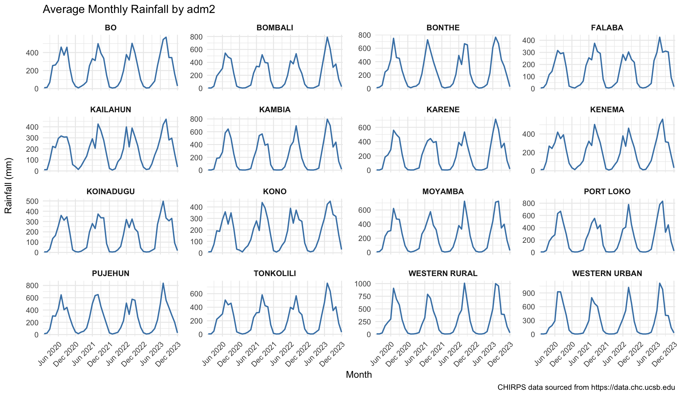
Step 4: Visualize Monthly Rainfall Trends
Step 4.1: Prepare data for plotting
After extracting our chirps rainfall data, it’s important to visualise basic patterns before saving and using for future analysis. This step helps identify missing months, anomalous zeros, or outliers that could indicate data quality issues or extraction errors.
We start by plotting monthly total rainfall for a sample of districts to inspect temporal variation and assess whether rainfall seasonality aligns with what is known about local transmission dynamics.
To adapt the code:
- Line 6: Make sure adm0, adm1, adm2 match your shapefile columns.
- Line 8: Ensure chirps_rainfall_mean matches the column name generated by your processing. If you used a different aggregation or renamed the column, update accordingly.
- Line 4: year_month is already created from year and month. You don’t need to change this unless your structure is different.
Once updated, run the code to prepare data for visualization.
Step 4.2: Visualise monthly rainfall trends
We plot monthly rainfall for a sample of districts to assess temporal variation.
Show the code
# plot CHIRPS monthly data
plot <- rain_plot_data |>
ggplot2::ggplot(ggplot2::aes(x = year_month, y = avg_mean_rain)) +
ggplot2::geom_line(linewidth = 0.8, color = "steelblue") +
ggplot2::scale_x_date(
date_breaks = "6 months",
date_labels = "%b %Y",
expand = c(0.01, 0.01)
) +
ggplot2::facet_wrap(~adm2, scales = "free_y", ncol = 4) +
ggplot2::labs(
title = "Average Monthly Rainfall by adm2",
x = "Month",
y = "Rainfall (mm)\n ",
caption = "CHIRPS data sourced from https://data.chc.ucsb.edu"
) +
ggplot2::theme_minimal(base_size = 12) +
ggplot2::theme(
strip.text = ggplot2::element_text(face = "bold", size = 10),
axis.text.x = ggplot2::element_text(angle = 45, hjust = 1),
panel.spacing = ggplot2::unit(1, "lines")
)
plot
NoteOutput
To adapt the code:
- Line 3: year_month should already exist in your dataset; avg_mean_rain should be replaced if your rainfall column has a different name.
- Line 10:
facet_wrap(~ adm2)should replace adm2 with your desired administrative level (e.g., district, province, etc.). - Lines 11–15: Adjust the title text to reflect your region or variable of interest, and update the data source link or text if using a different dataset.
Once updated, run the code to generate the plot.
ImportantValidate with the SNT Team
Even if you are working with a gridded climate or environmental dataset for SNT, ask the SNT team whether they have access to any observational data from national meteorological or hydrological stations. Even when partial, this ground-based data provides a valuable benchmark for confirming the accuracy of satellite-derived inputs.
For example, raster layers like CHIRPS rainfall estimates or NDVI time series can be validated against observed station records to ensure that seasonal trends and spatial gradients reflect real conditions. These comparisons help ensure confidence in the data before applying it to epidemiological analysis, risk stratification, or GIS-based decision support.
Whether or not local meteorological data is available, still present the maps and time series from the raster extractions to the SNT team for discussion and validation before use in later analyses.
Now let us save this plot for future reference.
To adapt the code:
- Lines 4–5: Update the filename path to match your folder structure and change
chirps_seasonality_check_adm3_2020_2023.pngas needed. - Line 6: Adjust the width, height, and dpi if you need a different image size or quality.
Once updated, run the code to save the plot as a PNG file.
Step 5: Save Processed Rainfall Data
We save the cleaned and aggregated rainfall dataset for later use in the SNT seasonality analysis.
# define save path
# save processed file as CSV
rio::export(
chirps_final,
here::here(climate_path, "processed",
"chirps_rainfall_adm3_processed_2020_2023.csv")
)
# save processed file as RDS
rio::export(
chirps_final,
here::here(climate_path, "processed",
"chirps_rainfall_adm3_processed_2020_2023.rds")
)To adapt the code:
- Lines 6–7, 13–14: Update the file paths to match your output directory structure.
- File names: Change file names (e.g.,
chirps_rainfall_adm3_processed_2020_2023.csv) to reflect your dataset, time range, or administrative level.
Once updated, run the code to save your outputs in both raw and processed formats.
Summary
This section walked through the full process of generating monthly rainfall indicators using CHIRPS raster files: from downloading and inspecting high-resolution .tif data to extracting district-level statistics and visualizing seasonal trends. Remember to validate all outputs with the SNT team, presenting your maps and time series alongside any available station observations before integrating into downstream analyses. The complete pipeline is available at the end of this page for adaptation to your own shapefiles, regions, or time periods. Going through each of the data-processing steps carefully, especially extraction and visualization, ensures you know exactly which outputs must be validated by the SNT team.
Full Code
Find the full code script for climate and environmental data extraction from rasters below.
Show full code
################################################################################
###### ~ Climate and environment data extraction from raster full code ~ #######
################################################################################
### Step 1: Set-up and Download CHIRPS Raster Files ----------------------------
#### Step 1.1: Initial set-up --------------------------------------------------
# load required packages
pacman::p_load(
terra, # for raster operations
sf, # for vector data
exactextractr, # for precise extraction from rasters
dplyr, # for data manipulation
lubridate, # for date handling
here # for file path management
)
# download latest sntutils if you haven't already
devtools::install_github("ahadi-analytics/sntutils")
# import administrative boundary shapefile
sl_adm3_shp <- readRDS(
here::here("01_foundational/1a_administrative_boundaries",
"1ai_adm3", "sle_spatial_adm3_2021.rds")
) |> sf::st_as_sf() # ensure it gets turned into sf format
#### Step 1.2: Check available CHIRPS datasets ---------------------------------
# check available CHIRPS data to download
sntutils::chirps_options()
# check available years and months for africa_monthly dataset
sntutils::check_chirps_available("africa_monthly")
#### Step 1.3: Download CHIRPS raster data -------------------------------------
# set main climate data path
climate_path <- "05_climate_and environment"

# download CHIRPS data for 2020-2023
sntutils::download_chirps(dataset = "africa_monthly",
                             start = "2020-01",
                             end = "2023-12",
                             out_dir = here::here(climate_path, "raw"))
### Step 2: Load, Inspect, and Process a Single CHIRPS Raster ------------------
#### Step 2.1: Load and clean the raster ---------------------------------------
# read CHIRPS raster in May 2023
chirps_may2023 <- terra::rast(
 x = here::here(climate_path, "raw",
             "africa_monthly_chirps-v2.0.2023.05.tif")
)

# drop the missing values
chirps_may2023[chirps_may2023 == -9999] <- NA
#### Step 2.2: Visualize the raster --------------------------------------------
# plots raster
terra::plot(chirps_may2023)
#### Step 2.3: Extract rainfall values from rasters ----------------------------
# align CRS if needed
sl_adm3_shp <- sf::st_transform(sl_adm3_shp,
                                terra::crs(chirps_may2023))

# extract mean and sum rainfall
zonal_stats <- exactextractr::exact_extract(
  chirps_may2023,
  sl_adm3_shp,
  fun = c("mean"),
  progress = FALSE
)
#### Step 2.4: Combine with attributes and format output -----------------------
# bind extracted values to admin attributes and format output
result_df <- cbind(sl_adm3_shp, as.data.frame(zonal_stats)) |>
  dplyr::mutate(
    year = 2023,
    month = 5,
    chirps_mean = mean
  ) |>
  dplyr::select(adm0, adm1, adm2, adm3,
                year, month,
                chirps_mean) |>
  sf::st_drop_geometry()

# preview results for May 2023
head(result_df)
### Step 3: Batch Process All Raster Files -------------------------------------
# import administrative boundary shapefile
chirps_all <- sntutils::process_raster_collection(
  directory = "05_climate_and environment/raw",
  shapefile = sl_adm3_shp,
  id_cols = c("adm0", "adm1", "adm2", "adm3"),
  aggregations = c("mean"),
  pattern = ".tif"
)

# clean up the dataset
chirps_final <- chirps_all |>
  dplyr::rename(
    chirps_rainfall_mean = mean,
  ) |>
  dplyr::select(-file_name)

# check head
chirps_final |>
  dplyr::filter(year == 2023 & month == 05) |>
  head()
### Step 4: Visualize Monthly Rainfall Trends ----------------------------------
#### Step 4.1: Prepare data for plotting ---------------------------------------
# prepare data for plotting
rain_plot_data <- chirps_final |>
  dplyr::mutate(
    year_month = lubridate::make_date(year, month, 1)
  ) |>
  dplyr::group_by(adm0, adm1, adm2, year_month) |>
  dplyr::summarise(
    avg_mean_rain = mean(chirps_rainfall_mean, na.rm = TRUE),
    .groups = 'drop')
#### Step 4.2: Visualise monthly rainfall trends -------------------------------
# plot CHIRPS monthly data
plot <- rain_plot_data |>
  ggplot2::ggplot(ggplot2::aes(x = year_month, y = avg_mean_rain)) +
  ggplot2::geom_line(linewidth = 0.8, color = "steelblue") +
  ggplot2::scale_x_date(
    date_breaks = "6 months",
    date_labels = "%b %Y",
    expand = c(0.01, 0.01)
  ) +
  ggplot2::facet_wrap(~adm2, scales = "free_y", ncol = 4) +
  ggplot2::labs(
    title = "Average Monthly Rainfall by adm2",
    x = "Month",
    y = "Rainfall (mm)\n ",
    caption = "CHIRPS data sourced from https://data.chc.ucsb.edu"
  ) +
  ggplot2::theme_minimal(base_size = 12) +
  ggplot2::theme(
    strip.text = ggplot2::element_text(face = "bold", size = 10),
    axis.text.x = ggplot2::element_text(angle = 45, hjust = 1),
    panel.spacing = ggplot2::unit(1, "lines")
  )

plot
# save plot
ggplot2::ggsave(
  plot = plot,
  here::here("03_output/3a_figures",
             "chirps_seasonality_check_adm3_2020_2023.png"),
  width = 12, height = 7, dpi = 300
)
### Step 5: Save Processed Rainfall Data ---------------------------------------
# define save path

# save processed file as CSV
rio::export(
  chirps_final,
  here::here(climate_path, "processed",
             "chirps_rainfall_adm3_processed_2020_2023.csv")
)

# save processed file as RDS
rio::export(
  chirps_final,
  here::here(climate_path, "processed",
             "chirps_rainfall_adm3_processed_2020_2023.rds")
)