Routine intervention
Overview
The Expanded Programme on Immunization (EPI) plays a vital role in protecting communities from vaccine-preventable diseases through routine health facility–based and outreach interventions. These interventions ensure that essential vaccines and maternal–child health services are delivered consistently throughout the year, rather than only during campaigns. Routine EPI services typically include childhood immunizations (such as BCG, Pentavalent, Measles), maternal health interventions (such as Antenatal Care and Intermittent Preventive Treatment in Pregnancy), and child survival programs (such as Vitamin A supplementation and Long-Lasting Insecticidal Net distribution).
Monitoring and analyzing these routine data are essential for identifying coverage gaps, understanding service performance across districts, and supporting national efforts to improve health outcomes. By processing and harmonizing routine EPI data from health facilities, this analysis provides a reliable foundation for tracking progress, evaluating program effectiveness, and guiding strategic planning at both district and national levels.
- Standardize and consolidate routine EPI data from multiple districts (2015–2023) into a unified, analyzable format.
- Calculate coverage and dropout rates for key interventions such as Pentavalent (Penta1, Penta3), Measles, IPTi, IPT, Vitamin A, ANC, and LLIN distribution.
- Integrate facility-based and outreach data to generate accurate estimates of total interventions delivered.
- Summarize performance by administrative level and year, enabling data-driven comparisons across time and regions.
- Produce a clean, comprehensive dataset to support visualization, mapping, and statistical analyses that inform immunization program improvements.
Step-by-Step
To skip the step-by-step explanation, jump to the full code at the end of this page.
Step 1: Install and load packages
To adapt the code:
- Do not change anything in the code
Step 2: Read and combine district files
To adapt the code:
- Line 2: Update folder path to your data location
Step 3: Process date column
month_map <- base::c(
"January" = "01", "February" = "02", "March" = "03",
"April" = "04", "May" = "05", "June" = "06",
"July" = "07", "August" = "08", "September" = "09",
"October" = "10", "November" = "11", "December" = "12"
)
epi_data <- epi_data |>
tidyr::separate(
periodname,
into = c("month_name", "year"),
sep = " ",
remove = FALSE
) |>
dplyr::mutate(
month = month_map[month_name],
year = base::as.numeric(year),
date = base::paste(year, month, sep = "-")
)To adapt the code:
- Lines 2-6: Translate month names if different language
- Line 10: Change
periodnameto your date column name
Step 4: Rename columns
Step 5: Calculate intervention totals
# Penta
epi_data$penta1 <- rowSums(epi_data[, c('Pentavalent 1st dose In_Facility_X, 0-11m_X', 'Pentavalent 1st dose Outreach_X, 0-11m_X')], na.rm = TRUE)
epi_data$penta3 <- rowSums(epi_data[, c('Pentavalent 3rd dose In_Facility_X, 0-11m_X', 'Pentavalent 3rd dose Outreach_X, 0-11m_X')], na.rm = TRUE)
# LLINs given during penta3 and anc
epi_data$llins_given_during_penta3 <- rowSums(epi_data[, c('LLITN given at Pentavalent 3rd dose In_Facility_X, 0-11m_X', 'LLITN given at Pentavalent 3rd dose Outreach_X, 0-11m_X')], na.rm = TRUE)
epi_data$llins_given_during_anc <- rowSums(epi_data[, c('Antenatal client given LLITN In_Facility_X', 'Antenatal client given LLITN Outreach_X')], na.rm = TRUE)
# Measles
epi_data$measles_infants <- rowSums(epi_data[, c('Measles 1st dose In_Facility_X, 0-11m_X', 'Measles 1st dose Outreach_X, 0-11m_X')], na.rm = TRUE)
epi_data$measles_child <- rowSums(epi_data[, c('Measles 1st dose In_Facility_X, 12-59m_X', 'Measles 1st dose Outreach_X, 12-59m_X')], na.rm = TRUE)
# IPTi
epi_data$ipti1 <- rowSums(epi_data[, c('IPTi 1st dose given In_Facility_X, 0-11m_X', 'IPTi 1st dose given Outreach_X, 0-11m_X')], na.rm = TRUE)
epi_data$ipti2 <- rowSums(epi_data[, c('IPTi 2nd dose given In_Facility_X, 0-11m_X', 'IPTi 2nd dose given Outreach_X, 0-11m_X')], na.rm = TRUE)
epi_data$ipti3 <- rowSums(epi_data[, c('IPTi 3rd dose given In_Facility_X, 0-11m_X', 'IPTi 3rd dose given Outreach_X, 0-11m_X')], na.rm = TRUE)
# ANC
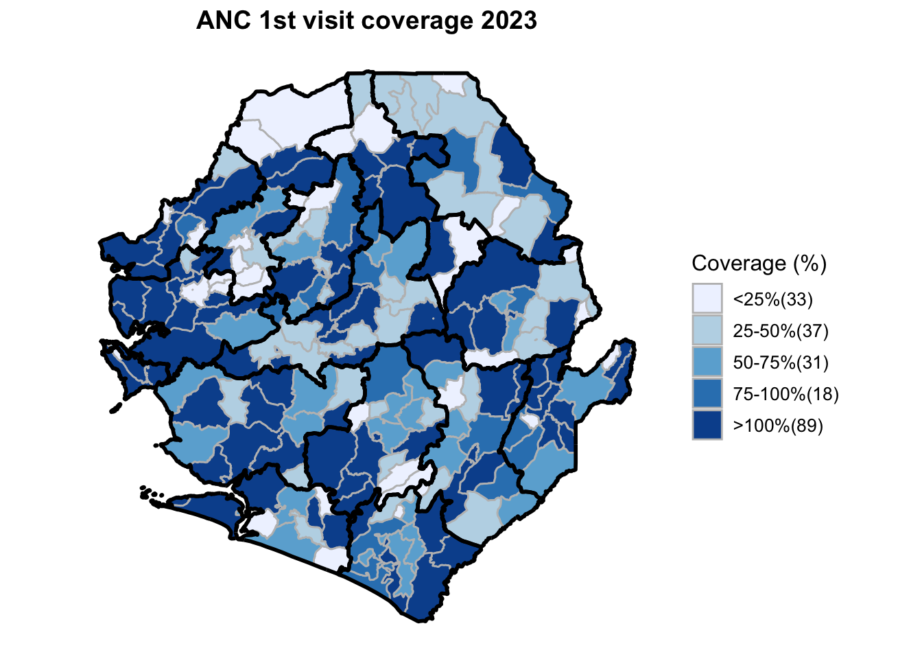
epi_data$anc1 <- rowSums(epi_data[, c('Antenatal client 1st visit In_Facility_X', 'Antenatal client 1st visit Outreach_X')], na.rm = TRUE)
epi_data$anc4 <- rowSums(epi_data[, c('Antenatal client 4th visit In_Facility_X', 'Antenatal client 4th visit Outreach_X')], na.rm = TRUE)
epi_data$anc8 <- rowSums(epi_data[, c('Antenatal client 8th visit In_Facility_X', 'Antenatal client 8th visit Outreach_X')], na.rm = TRUE)
# IPT
epi_data$ipt1 <- rowSums(epi_data[, c('Antenatal client IPT 1st dose In_Facility_X', 'Antenatal client IPT 1st dose Outreach_X')], na.rm = TRUE)
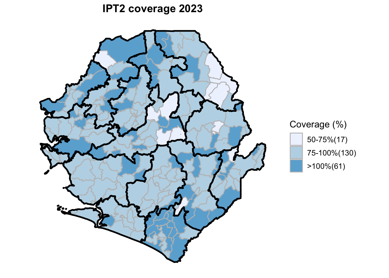
epi_data$ipt2 <- rowSums(epi_data[, c('Antenatal client IPT 2nd dose In_Facility_X', 'Antenatal client IPT 2nd dose Outreach_X')], na.rm = TRUE)
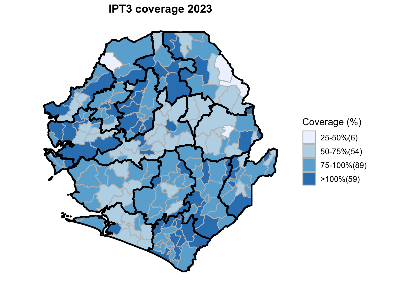
epi_data$ipt3 <- rowSums(epi_data[, c('Antenatal client IPT 3rd dose In_Facility_X', 'Antenatal client IPT 3rd dose Outreach_X')], na.rm = TRUE)
# Vitamin A
epi_data$vitamin_infants <- rowSums(epi_data[, c('Vitamin A supplement 6-11 months In_Facility_X', 'Vitamin A supplement 6-11 months Outreach_X')], na.rm = TRUE)
epi_data$vitamin_child <- rowSums(epi_data[, c('Vitamin A supplement 12-59 months In_Facility_X', 'Vitamin A supplement 12-59 months Outreach_X')], na.rm = TRUE)To adapt the code:
- Line 4-32: Update the exact column names in quotes to match your dataset’s column names
Step 6: Import population data
Step 7: Aggregate by year
intervention_cols <- base::c(
"penta1", "penta3", "ipti1", "ipti2", "ipti3",
"ipt1", "ipt2", "ipt3", "vitamin_infants", "vitamin_child",
"measles_infants", "measles_child", "anc1", "anc4", "anc8",
"llins_given_during_anc", "llins_given_during_penta3"
)
yearly_data <- base::list()
for (yr in 2015:2023) {
yearly_data[[base::as.character(yr)]] <- epi_data |>
dplyr::filter(year == yr) |>
dplyr::group_by(adm1, adm2, adm3) |>
dplyr::summarise(
dplyr::across(dplyr::all_of(intervention_cols), ~base::sum(.x, na.rm = TRUE)),
.groups = "drop"
) |>
dplyr::rename_with(~base::paste0(.x, "_", yr), dplyr::all_of(intervention_cols))
}
epi_merged <- purrr::reduce(yearly_data, dplyr::full_join, by = base::c("adm1", "adm2", "adm3"))To adapt the code:
- Lines 2-6: Update intervention list
- Line 10: Change year range
- Line 13: Adjust admin levels
Step 8: Calculate coverage rates
Show the code
for (yr in 2015:2023) {
pop_col <- base::paste0("pop", yr)
if (!pop_col %in% base::names(pop_data)) next
# Penta1 coverage
epi_merged[[base::paste0("penta1_coverage_", yr)]] <- base::round(
(epi_merged[[base::paste0("penta1_", yr)]] / (pop_data[[pop_col]] * 0.037)) * 100, 2
)
# Penta3 coverage
epi_merged[[base::paste0("penta3_coverage_", yr)]] <- base::ifelse(
base::is.na(epi_merged[[base::paste0("penta1_", yr)]]) | epi_merged[[base::paste0("penta1_", yr)]] == 0,
0,
base::round((epi_merged[[base::paste0("penta3_", yr)]] / epi_merged[[base::paste0("penta1_", yr)]]) * 100, 2)
)
# IPTi1 coverage
epi_merged[[base::paste0("ipti1_coverage_", yr)]] <- base::round(
(epi_merged[[base::paste0("ipti1_", yr)]] / (pop_data[[pop_col]] * 0.037)) * 100, 2
)
# IPTi2 coverage
epi_merged[[base::paste0("ipti2_coverage_", yr)]] <- base::ifelse(
base::is.na(epi_merged[[base::paste0("ipti1_", yr)]]) | epi_merged[[base::paste0("ipti1_", yr)]] == 0,
0,
base::round((epi_merged[[base::paste0("ipti2_", yr)]] / epi_merged[[base::paste0("ipti1_", yr)]]) * 100, 2)
)
# IPTi3 coverage
epi_merged[[base::paste0("ipti3_coverage_", yr)]] <- base::ifelse(
base::is.na(epi_merged[[base::paste0("ipti1_", yr)]]) | epi_merged[[base::paste0("ipti1_", yr)]] == 0,
0,
base::round((epi_merged[[base::paste0("ipti3_", yr)]] / epi_merged[[base::paste0("ipti1_", yr)]]) * 100, 2)
)
# IPT1 coverage
epi_merged[[base::paste0("ipt1_coverage_", yr)]] <- base::round(
(epi_merged[[base::paste0("ipt1_", yr)]] / (pop_data[[pop_col]] * 0.037)) * 100, 2
)
# IPT2 coverage
epi_merged[[base::paste0("ipt2_coverage_", yr)]] <- base::ifelse(
base::is.na(epi_merged[[base::paste0("ipt1_", yr)]]) | epi_merged[[base::paste0("ipt1_", yr)]] == 0,
0,
base::round((epi_merged[[base::paste0("ipt2_", yr)]] / epi_merged[[base::paste0("ipt1_", yr)]]) * 100, 2)
)
# IPT3 coverage
epi_merged[[base::paste0("ipt3_coverage_", yr)]] <- base::ifelse(
base::is.na(epi_merged[[base::paste0("ipt1_", yr)]]) | epi_merged[[base::paste0("ipt1_", yr)]] == 0,
0,
base::round((epi_merged[[base::paste0("ipt3_", yr)]] / epi_merged[[base::paste0("ipt1_", yr)]]) * 100, 2)
)
# Vitamin A infants coverage
epi_merged[[base::paste0("vitamin_infants_coverage_", yr)]] <- base::ifelse(
base::is.na(epi_merged[[base::paste0("vitamin_infants_", yr)]]) | base::is.na(pop_data[[pop_col]]),
0,
base::round((epi_merged[[base::paste0("vitamin_infants_", yr)]] / (pop_data[[pop_col]] * 0.02)) * 100, 2)
)
# Vitamin A child coverage
epi_merged[[base::paste0("vitamin_child_coverage_", yr)]] <- base::ifelse(
base::is.na(epi_merged[[base::paste0("vitamin_child_", yr)]]) | base::is.na(pop_data[[pop_col]]),
0,
base::round((epi_merged[[base::paste0("vitamin_child_", yr)]] / (pop_data[[pop_col]] * 0.137)) * 100, 2)
)
# Measles infants coverage
epi_merged[[base::paste0("measles_infants_coverage_", yr)]] <- base::ifelse(
base::is.na(epi_merged[[base::paste0("measles_infants_", yr)]]) | base::is.na(pop_data[[pop_col]]),
0,
base::round((epi_merged[[base::paste0("measles_infants_", yr)]] / (pop_data[[pop_col]] * 0.037)) * 100, 2)
)
# Measles child coverage
epi_merged[[base::paste0("measles_child_coverage_", yr)]] <- base::ifelse(
base::is.na(epi_merged[[base::paste0("measles_child_", yr)]]) | base::is.na(pop_data[[pop_col]]),
0,
base::round((epi_merged[[base::paste0("measles_child_", yr)]] / (pop_data[[pop_col]] * 0.137)) * 100, 2)
)
# ANC1 coverage
epi_merged[[base::paste0("anc1_coverage_", yr)]] <- base::round(
(epi_merged[[base::paste0("anc1_", yr)]] / (pop_data[[pop_col]] * 0.044)) * 100, 2
)
# ANC4 coverage
epi_merged[[base::paste0("anc4_coverage_", yr)]] <- base::ifelse(
base::is.na(epi_merged[[base::paste0("anc1_", yr)]]) | epi_merged[[base::paste0("anc1_", yr)]] == 0,
0,
base::round((epi_merged[[base::paste0("anc4_", yr)]] / epi_merged[[base::paste0("anc1_", yr)]]) * 100, 2)
)
# ANC8 coverage
epi_merged[[base::paste0("anc8_coverage_", yr)]] <- base::ifelse(
base::is.na(epi_merged[[base::paste0("anc1_", yr)]]) | epi_merged[[base::paste0("anc1_", yr)]] == 0,
0,
base::round((epi_merged[[base::paste0("anc8_", yr)]] / epi_merged[[base::paste0("anc1_", yr)]]) * 100, 2)
)
# LLINs during ANC coverage
epi_merged[[base::paste0("llins_anc_coverage_", yr)]] <- base::ifelse(
base::is.na(epi_merged[[base::paste0("anc1_", yr)]]) | epi_merged[[base::paste0("anc1_", yr)]] == 0,
0,
base::round((epi_merged[[base::paste0("llins_given_during_anc_", yr)]] / epi_merged[[base::paste0("anc1_", yr)]]) * 100, 2)
)
# LLINs during Penta3 coverage
epi_merged[[base::paste0("llins_penta3_coverage_", yr)]] <- base::ifelse(
base::is.na(epi_merged[[base::paste0("penta3_", yr)]]) | epi_merged[[base::paste0("penta3_", yr)]] == 0,
0,
base::round((epi_merged[[base::paste0("llins_given_during_penta3_", yr)]] / epi_merged[[base::paste0("penta3_", yr)]]) * 100, 2)
)
# Penta dropout rate
epi_merged[[base::paste0("penta_dropout_rate_", yr)]] <- base::ifelse(
base::is.na(epi_merged[[base::paste0("penta1_", yr)]]) | epi_merged[[base::paste0("penta1_", yr)]] == 0,
0,
base::round(((epi_merged[[base::paste0("penta1_", yr)]] - epi_merged[[base::paste0("penta3_", yr)]]) / epi_merged[[base::paste0("penta1_", yr)]]) * 100, 2)
)
# IPTi dropout rate
epi_merged[[base::paste0("ipti_dropout_rate_", yr)]] <- base::ifelse(
base::is.na(epi_merged[[base::paste0("ipti1_", yr)]]) | epi_merged[[base::paste0("ipti1_", yr)]] == 0,
0,
base::round(((epi_merged[[base::paste0("ipti1_", yr)]] - epi_merged[[base::paste0("ipti3_", yr)]]) / epi_merged[[base::paste0("ipti1_", yr)]]) * 100, 2)
)
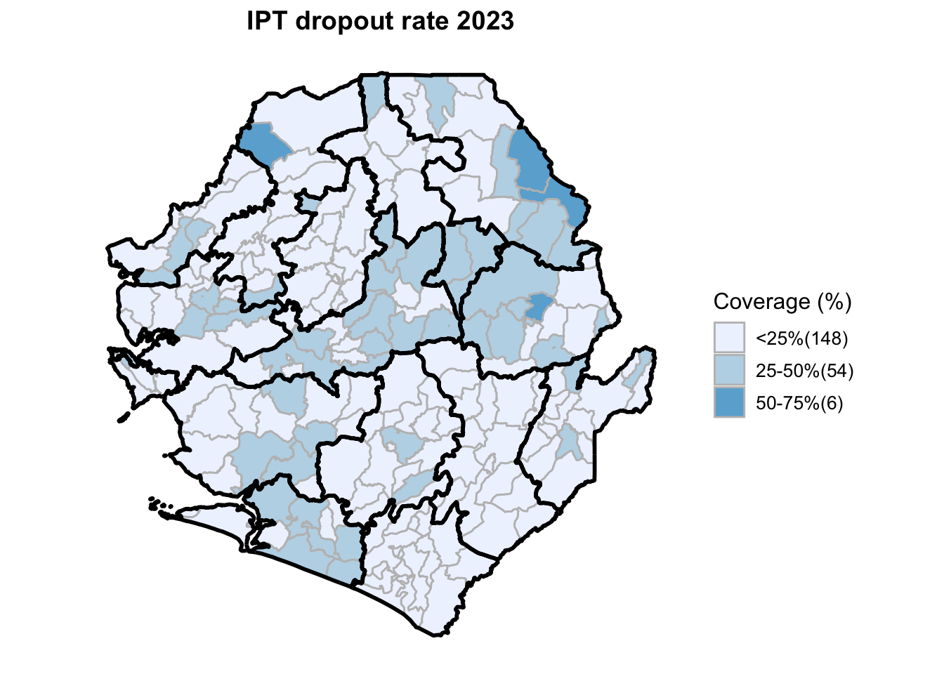
# IPT dropout rate
epi_merged[[base::paste0("ipt_dropout_rate_", yr)]] <- base::ifelse(
base::is.na(epi_merged[[base::paste0("ipt1_", yr)]]) | epi_merged[[base::paste0("ipt1_", yr)]] == 0,
0,
base::round(((epi_merged[[base::paste0("ipt1_", yr)]] - epi_merged[[base::paste0("ipt3_", yr)]]) / epi_merged[[base::paste0("ipt1_", yr)]]) * 100, 2)
)
# ANC dropout rate
epi_merged[[base::paste0("anc_dropout_rate_", yr)]] <- base::ifelse(
base::is.na(epi_merged[[base::paste0("anc1_", yr)]]) | epi_merged[[base::paste0("anc1_", yr)]] == 0,
0,
base::round(((epi_merged[[base::paste0("anc1_", yr)]] - epi_merged[[base::paste0("anc8_", yr)]]) / epi_merged[[base::paste0("anc1_", yr)]]) * 100, 2)
)
}To adapt the code:
Line 1: Change year range
Lines with population factors (0.037, 0.02, 0.137, 0.044): Adjust based on your demographic data
Step 9: Display the data and save
# Save to Excel file
#writexl::write_xlsx(epi_merged, here::here("past_intervention_coverage_processed_data.xlsx"))
epi_merged |>
head() |>
knitr::kable("html", caption = "Preview of epi_merged dataset") |>
kableExtra::kable_styling(bootstrap_options = c("striped", "hover", "condensed", "responsive"))To adapt the code:
- Line 2: Update output file path
Step 10: Load intervention data
To adapt the code:
- Line 1: Update file path to match your processed data location
Step 11: Load shapefiles
# Load chiefdom level shapefile (admin level 3)
shapefile_chiefdom <- readRDS(
here::here("data/shapefiles/processed/sle_spatial_adm3_2021.rds")
) |>
sf::st_as_sf()
# Load district level shapefile (admin level 2) for boundaries
shapefile_district <- readRDS(
here::here("data/shapefiles/processed/sle_spatial_adm2_2021.rds")
) |>
sf::st_as_sf()To adapt the code:
- Line 2: Update chiefdom shapefile path and filename
- Line 5: Update district shapefile path and filename
Step 12: Load merge key
Step 13: Merge datasets
# Merge intervention data with key file
epi_merged <- base::merge(epi_merged, key_file, by = "adm3", all.x = TRUE)
# Merge with chiefdom shapefile (shapefile uses adm2/adm3; key file uses FIRST_DNAM/FIRST_CHIE)
data <- base::merge(shapefile_chiefdom, epi_merged, by.x = base::c("adm2", "adm3"), by.y = base::c("FIRST_DNAM", "FIRST_CHIE"), all.x = TRUE)To adapt the code:
Line 2: Update merge keys to match your administrative level columns
Line 5: Update shapefile column names (FIRST_DNAM, FIRST_CHIE) to match your shapefile attributes
Step 14: Define visualization parameters
To adapt the code:
Line 1: Change color palette (e.g., “Reds”, “Greens”, “YlOrRd”)
Lines 3-11: Update columns to match your intervention indicators
Lines 13-21: Update titles to match your indicators
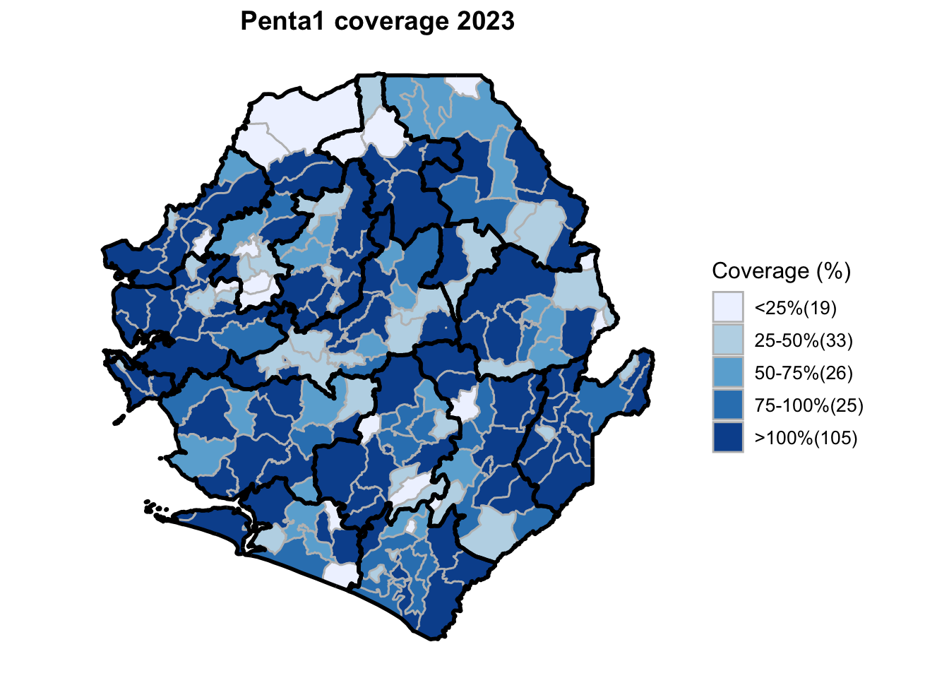
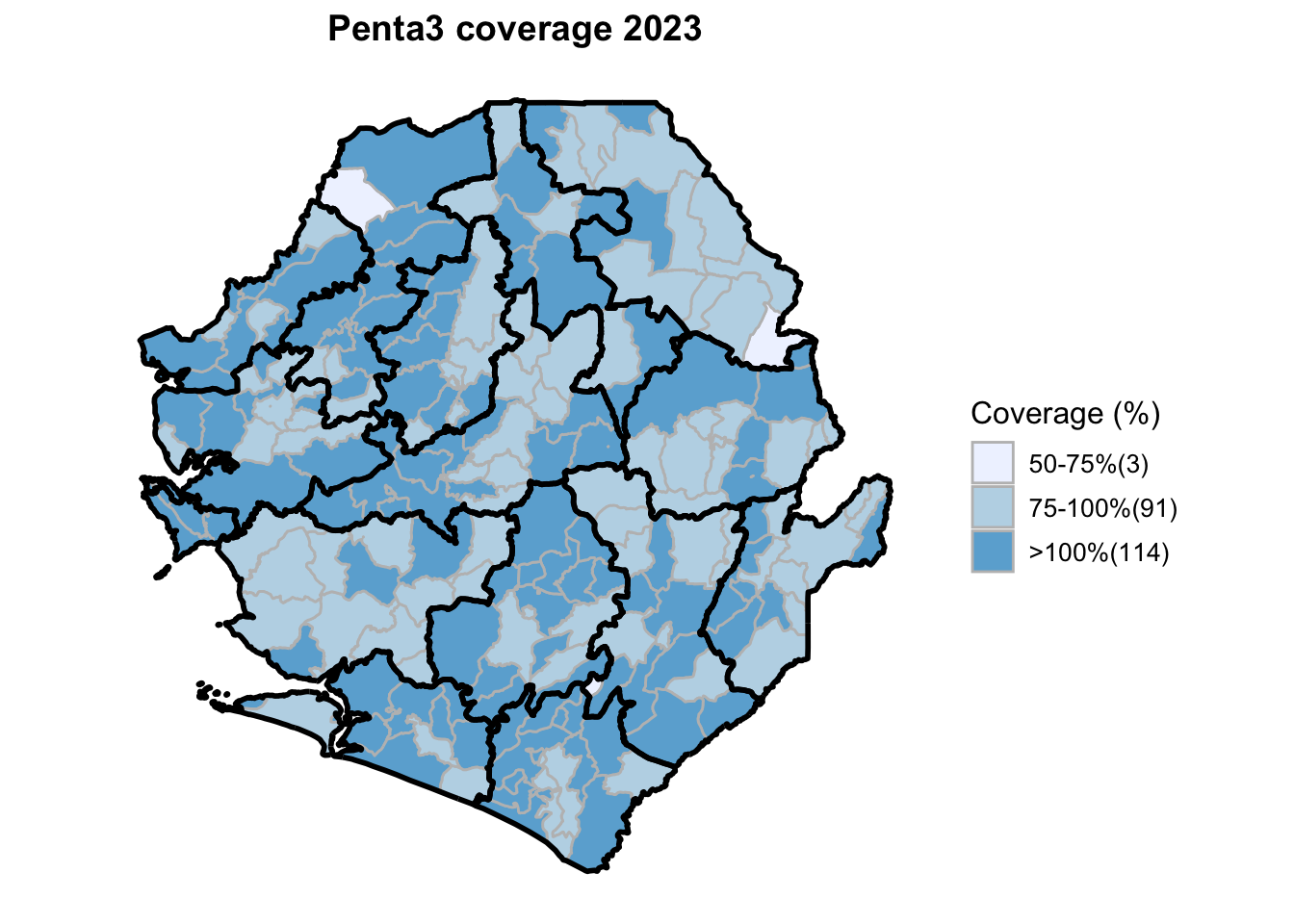
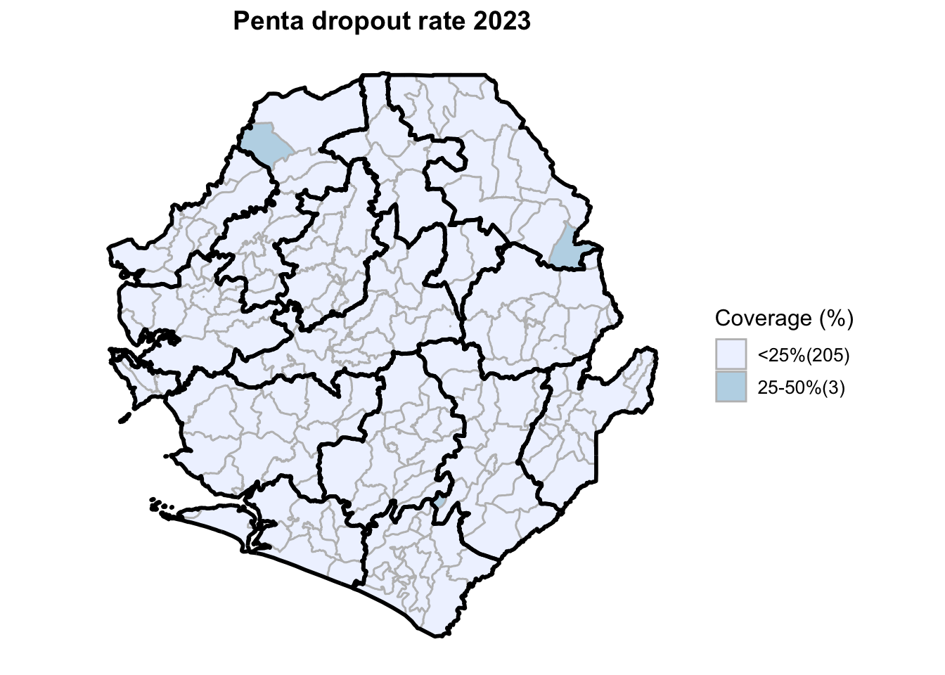
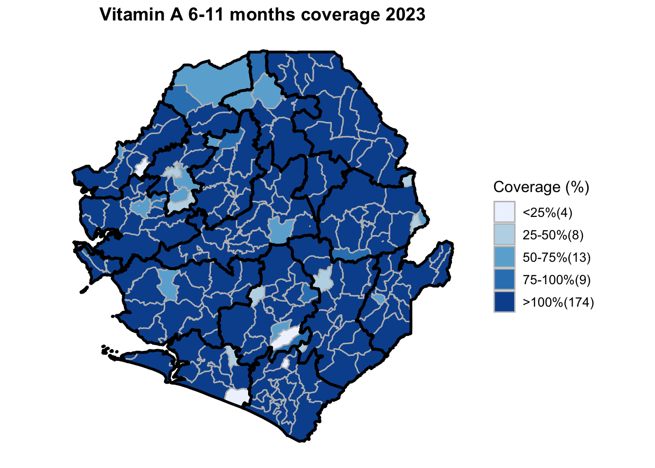
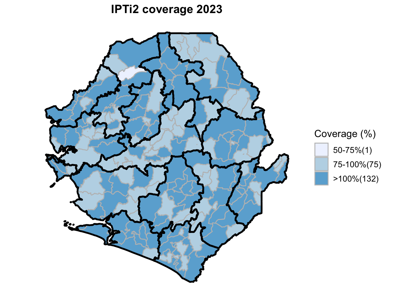
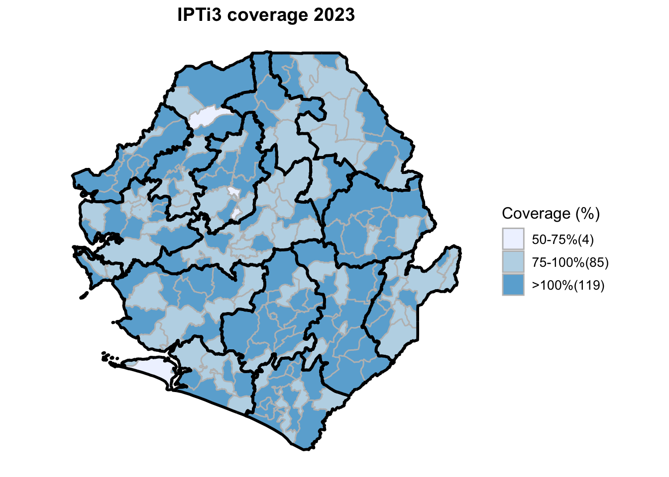
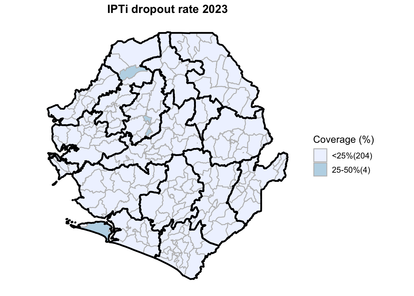
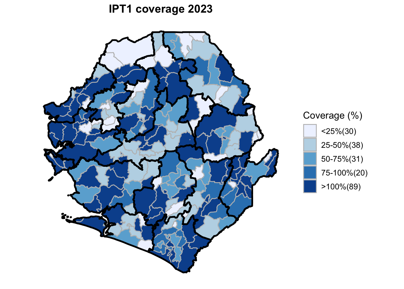
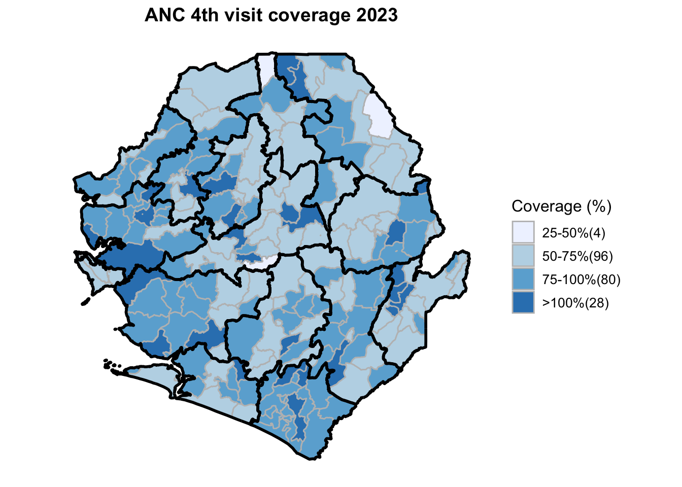
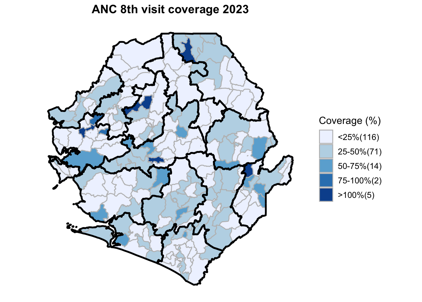
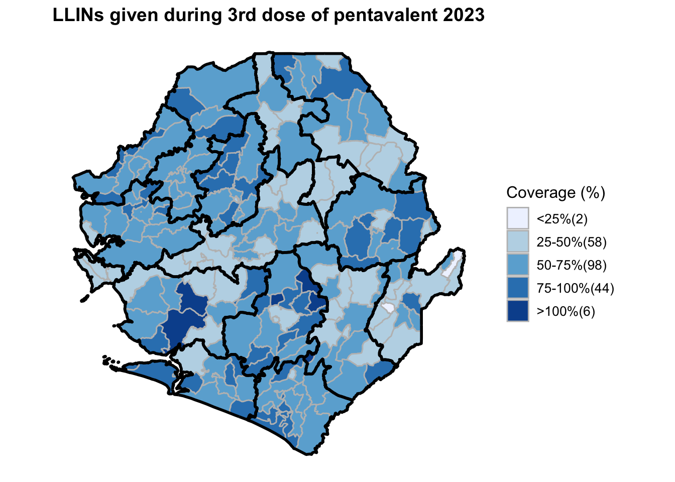
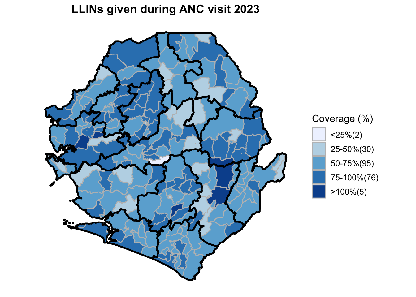
Step 15: Generate maps
Show the code
year <- 2023
for (col_index in base::seq_along(columns_to_plot)) {
coverage_prefix <- columns_to_plot[col_index]
plot_title <- titles[col_index]
coverage_col <- base::paste0(coverage_prefix, "_", year)
if (!(coverage_col %in% base::names(data))) {
base::print(base::paste("Skipping", coverage_col, "- column not found"))
next
}
data[[coverage_col]] <- base::as.numeric(base::as.character(data[[coverage_col]]))
data[[coverage_col]][base::is.na(data[[coverage_col]])] <- 0
data$coverage_category <- base::cut(
data[[coverage_col]],
breaks = base::c(-Inf, 25, 50, 75, 100, Inf),
labels = base::c("<25%", "25-50%", "50-75%", "75-100%", ">100%"),
include.lowest = TRUE
)
counts <- data |>
dplyr::group_by(coverage_category) |>
dplyr::summarise(count = dplyr::n()) |>
dplyr::ungroup()
non_zero_counts <- counts[counts$count > 0, ]
labels_with_counts <- base::paste(non_zero_counts$coverage_category, "(", non_zero_counts$count, ")", sep = "")
data$coverage_category <- base::factor(
data$coverage_category,
levels = base::c("<25%", "25-50%", "50-75%", "75-100%", ">100%")
)
plot <- ggplot2::ggplot(data) +
# Add chiefdom polygons with fill colors
ggplot2::geom_sf(ggplot2::aes(fill = coverage_category), color = "gray", linewidth= 0.5) +
# Add district boundaries as thicker lines
ggplot2::geom_sf(data = shapefile_district, fill = NA, color = "black", linewidth = 1.0 ) +
ggplot2::scale_fill_manual(
values = colors[1:base::length(non_zero_counts$coverage_category)],
breaks = non_zero_counts$coverage_category,
labels = labels_with_counts,
name = "Coverage (%)"
) +
ggplot2::labs(title = base::paste(plot_title, year)) +
ggplot2::theme_minimal() +
ggplot2::theme(
plot.title = ggplot2::element_text(size = 14, face = "bold", hjust = 0.5),
legend.title = ggplot2::element_text(size = 12),
legend.text = ggplot2::element_text(size = 10),
legend.position = "right",
panel.grid = ggplot2::element_blank(),
axis.text = ggplot2::element_blank(),
axis.ticks = ggplot2::element_blank()
)
base::print(plot)
}
To adapt the code:
Line 1: Change year to visualize different time periods (e.g., 2015-2023)
Lines 18-21: Adjust coverage breaks to suit your data ranges (currently: <25%, 25-50%, 50-75%, 75-100%, >100%)
Line 40: Modify chiefdom border color (gray60) and thickness (0.3)
Line 42: Modify district boundary color (black) and thickness (1.2) - thicker lines for district boundaries
Lines 50-57: Customize plot appearance (title size, legend position)
Summary
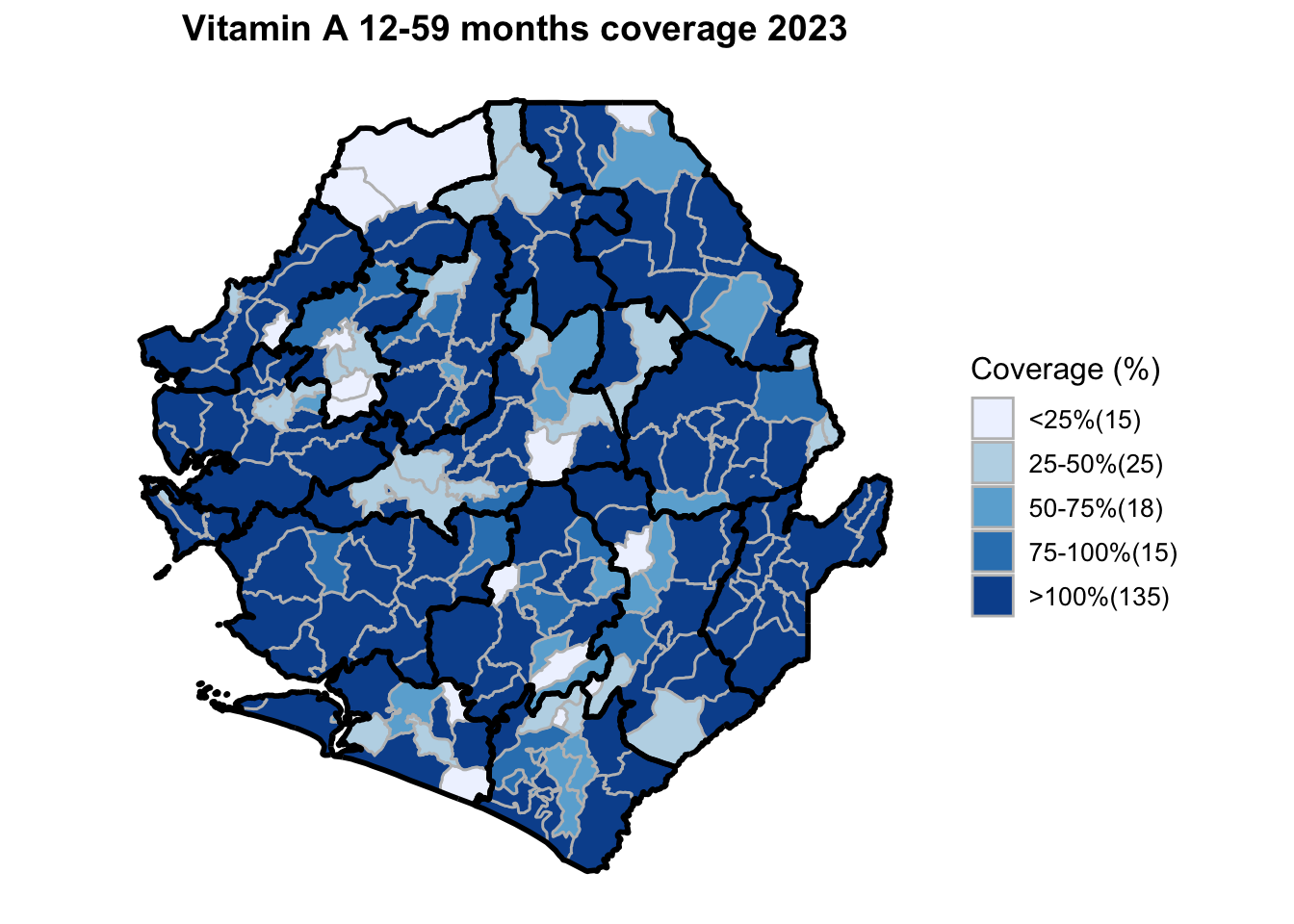
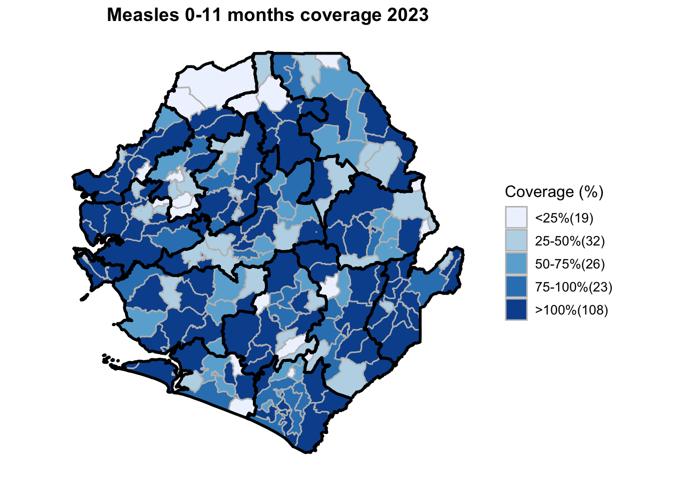
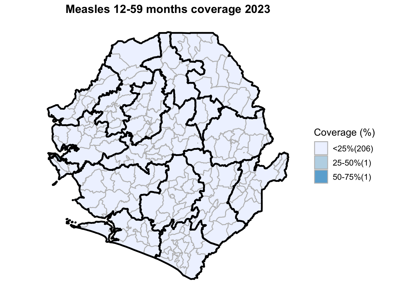
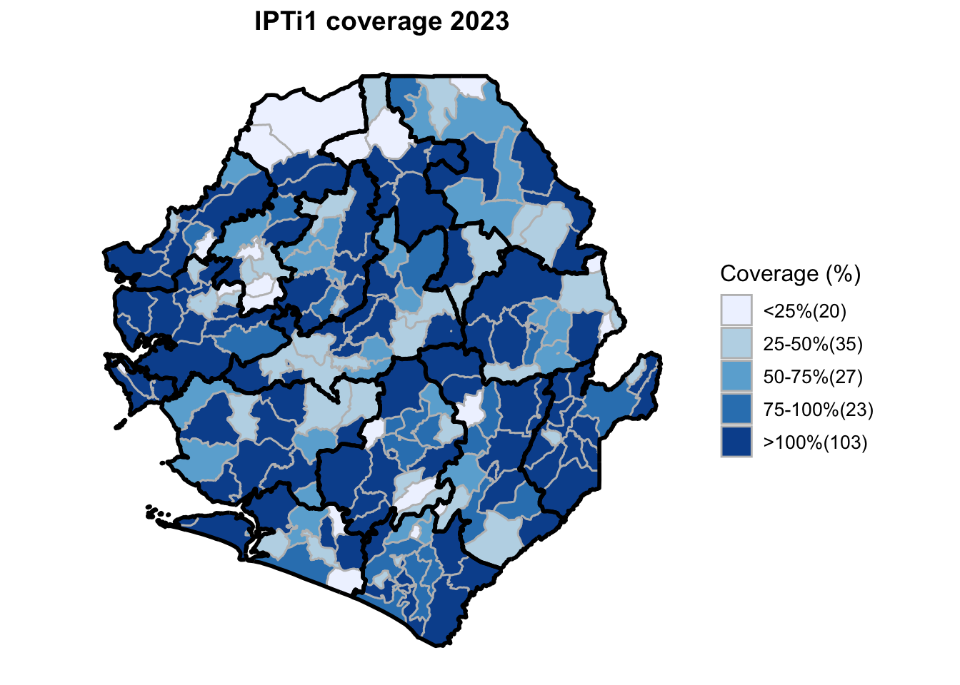
This workflow processes routine EPI intervention data from 2015 to 2023 across multiple districts, combining facility-based and outreach services to calculate comprehensive coverage and dropout rates. The analysis integrates district-level Excel files, standardizes date and administrative columns, computes intervention totals for key health services (Pentavalent, Measles, IPTi, IPT, Vitamin A, ANC, and LLIN distribution), and calculates population-adjusted coverage rates and dropout rates by chiefdom and year. The processed dataset is then merged with geographic shapefiles to generate choropleth maps visualizing coverage patterns across administrative regions, with district boundaries overlaid on chiefdom-level data. The final outputs include a comprehensive Excel file with annual intervention metrics and a series of maps showing geographic disparities in service delivery performance.
Full Code
Find the full code for routine EPI interventions below.
# ============================================================================
# PART A: DATA PROCESSING
# ============================================================================
# Step 1: Install and load packages
if (!base::requireNamespace("pacman", quietly = TRUE)) {
utils::install.packages("pacman")
}
pacman::p_load(
readxl, writexl, dplyr, tidyr, stringr, here, kableExtra,
sf, RColorBrewer, ggplot2
)
# Step 2: Read and combine district files
files <- base::list.files(
  path = here::here("english/data_r/intervention_data_recent"),
  pattern = "\\.xlsx$",
  full.names = TRUE
)

epi_data <- base::lapply(files, readxl::read_excel) |>
  dplyr::bind_rows()

base::names(epi_data) <- base::trimws(base::names(epi_data))
# Step 3: Process date column
month_map <- base::c(
  "January" = "01", "February" = "02", "March" = "03",
  "April" = "04", "May" = "05", "June" = "06",
  "July" = "07", "August" = "08", "September" = "09",
  "October" = "10", "November" = "11", "December" = "12"
)

epi_data <- epi_data |>
  tidyr::separate(
    periodname,
    into = c("month_name", "year"),
    sep = " ",
    remove = FALSE
  ) |>
  dplyr::mutate(
    month = month_map[month_name],
    year  = base::as.numeric(year),
    date  = base::paste(year, month, sep = "-")
  )
# Step 4: Rename columns
epi_data <- epi_data |>
  dplyr::rename(
    adm0 = orgunitlevel1,
    adm1 = orgunitlevel2,
    adm2 = orgunitlevel3,
    adm3 = orgunitlevel4,
    hf = organisationunitname
  )
# Step 5: Calculate intervention totals
# Penta
epi_data$penta1 <- rowSums(epi_data[, c('Pentavalent 1st dose In_Facility_X, 0-11m_X', 'Pentavalent 1st dose Outreach_X, 0-11m_X')], na.rm = TRUE)
epi_data$penta3 <- rowSums(epi_data[, c('Pentavalent 3rd dose In_Facility_X, 0-11m_X', 'Pentavalent 3rd dose Outreach_X, 0-11m_X')], na.rm = TRUE)

# LLINs given during penta3 and anc
epi_data$llins_given_during_penta3 <- rowSums(epi_data[, c('LLITN given at Pentavalent 3rd dose In_Facility_X, 0-11m_X', 'LLITN given at Pentavalent 3rd dose Outreach_X, 0-11m_X')], na.rm = TRUE)
epi_data$llins_given_during_anc <- rowSums(epi_data[, c('Antenatal client given LLITN In_Facility_X', 'Antenatal client given LLITN Outreach_X')], na.rm = TRUE)

# Measles
epi_data$measles_infants <- rowSums(epi_data[, c('Measles 1st dose In_Facility_X, 0-11m_X', 'Measles 1st dose Outreach_X, 0-11m_X')], na.rm = TRUE)
epi_data$measles_child <- rowSums(epi_data[, c('Measles 1st dose In_Facility_X, 12-59m_X', 'Measles 1st dose Outreach_X, 12-59m_X')], na.rm = TRUE)

# IPTi
epi_data$ipti1 <- rowSums(epi_data[, c('IPTi 1st dose given In_Facility_X, 0-11m_X', 'IPTi 1st dose given Outreach_X, 0-11m_X')], na.rm = TRUE)
epi_data$ipti2 <- rowSums(epi_data[, c('IPTi 2nd dose given In_Facility_X, 0-11m_X', 'IPTi 2nd dose given Outreach_X, 0-11m_X')], na.rm = TRUE)
epi_data$ipti3 <- rowSums(epi_data[, c('IPTi 3rd dose given In_Facility_X, 0-11m_X', 'IPTi 3rd dose given Outreach_X, 0-11m_X')], na.rm = TRUE)

# ANC
epi_data$anc1 <- rowSums(epi_data[, c('Antenatal client 1st visit In_Facility_X', 'Antenatal client 1st visit Outreach_X')], na.rm = TRUE)
epi_data$anc4 <- rowSums(epi_data[, c('Antenatal client 4th visit In_Facility_X', 'Antenatal client 4th visit Outreach_X')], na.rm = TRUE)
epi_data$anc8 <- rowSums(epi_data[, c('Antenatal client 8th visit In_Facility_X', 'Antenatal client 8th visit Outreach_X')], na.rm = TRUE)

# IPT
epi_data$ipt1 <- rowSums(epi_data[, c('Antenatal client IPT 1st dose In_Facility_X', 'Antenatal client IPT 1st dose Outreach_X')], na.rm = TRUE)
epi_data$ipt2 <- rowSums(epi_data[, c('Antenatal client IPT 2nd dose In_Facility_X', 'Antenatal client IPT 2nd dose Outreach_X')], na.rm = TRUE)
epi_data$ipt3 <- rowSums(epi_data[, c('Antenatal client IPT 3rd dose In_Facility_X', 'Antenatal client IPT 3rd dose Outreach_X')], na.rm = TRUE)

# Vitamin A
epi_data$vitamin_infants <- rowSums(epi_data[, c('Vitamin A supplement 6-11 months In_Facility_X', 'Vitamin A supplement 6-11 months Outreach_X')], na.rm = TRUE)
epi_data$vitamin_child <- rowSums(epi_data[, c('Vitamin A supplement 12-59 months In_Facility_X', 'Vitamin A supplement 12-59 months Outreach_X')], na.rm = TRUE)
# Step 6: Import population data
pop_data <- readxl::read_excel(here::here("english/data_r/pop/sle_pop_data.xlsx"))
# Step 7: Aggregate by year
intervention_cols <- base::c(
  "penta1", "penta3", "ipti1", "ipti2", "ipti3",
  "ipt1", "ipt2", "ipt3", "vitamin_infants", "vitamin_child",
  "measles_infants", "measles_child", "anc1", "anc4", "anc8",
  "llins_given_during_anc", "llins_given_during_penta3"
)

yearly_data <- base::list()

for (yr in 2015:2023) {
  yearly_data[[base::as.character(yr)]] <- epi_data |>
    dplyr::filter(year == yr) |>
    dplyr::group_by(adm1, adm2, adm3) |>
    dplyr::summarise(
      dplyr::across(dplyr::all_of(intervention_cols), ~base::sum(.x, na.rm = TRUE)),
      .groups = "drop"
    ) |>
    dplyr::rename_with(~base::paste0(.x, "_", yr), dplyr::all_of(intervention_cols))
}

epi_merged <- purrr::reduce(yearly_data, dplyr::full_join, by = base::c("adm1", "adm2", "adm3"))
# Step 8: Calculate coverage rates
for (yr in 2015:2023) {
  pop_col <- base::paste0("pop", yr)

  if (!pop_col %in% base::names(pop_data)) next

  # Penta1 coverage
  epi_merged[[base::paste0("penta1_coverage_", yr)]] <- base::round(
    (epi_merged[[base::paste0("penta1_", yr)]] / (pop_data[[pop_col]] * 0.037)) * 100, 2
  )

  # Penta3 coverage
  epi_merged[[base::paste0("penta3_coverage_", yr)]] <- base::ifelse(
    base::is.na(epi_merged[[base::paste0("penta1_", yr)]]) | epi_merged[[base::paste0("penta1_", yr)]] == 0,
    0,
    base::round((epi_merged[[base::paste0("penta3_", yr)]] / epi_merged[[base::paste0("penta1_", yr)]]) * 100, 2)
  )

  # IPTi1 coverage
  epi_merged[[base::paste0("ipti1_coverage_", yr)]] <- base::round(
    (epi_merged[[base::paste0("ipti1_", yr)]] / (pop_data[[pop_col]] * 0.037)) * 100, 2
  )

  # IPTi2 coverage
  epi_merged[[base::paste0("ipti2_coverage_", yr)]] <- base::ifelse(
    base::is.na(epi_merged[[base::paste0("ipti1_", yr)]]) | epi_merged[[base::paste0("ipti1_", yr)]] == 0,
    0,
    base::round((epi_merged[[base::paste0("ipti2_", yr)]] / epi_merged[[base::paste0("ipti1_", yr)]]) * 100, 2)
  )

  # IPTi3 coverage
  epi_merged[[base::paste0("ipti3_coverage_", yr)]] <- base::ifelse(
    base::is.na(epi_merged[[base::paste0("ipti1_", yr)]]) | epi_merged[[base::paste0("ipti1_", yr)]] == 0,
    0,
    base::round((epi_merged[[base::paste0("ipti3_", yr)]] / epi_merged[[base::paste0("ipti1_", yr)]]) * 100, 2)
  )

  # IPT1 coverage
  epi_merged[[base::paste0("ipt1_coverage_", yr)]] <- base::round(
    (epi_merged[[base::paste0("ipt1_", yr)]] / (pop_data[[pop_col]] * 0.037)) * 100, 2
  )

  # IPT2 coverage
  epi_merged[[base::paste0("ipt2_coverage_", yr)]] <- base::ifelse(
    base::is.na(epi_merged[[base::paste0("ipt1_", yr)]]) | epi_merged[[base::paste0("ipt1_", yr)]] == 0,
    0,
    base::round((epi_merged[[base::paste0("ipt2_", yr)]] / epi_merged[[base::paste0("ipt1_", yr)]]) * 100, 2)
  )

  # IPT3 coverage
  epi_merged[[base::paste0("ipt3_coverage_", yr)]] <- base::ifelse(
    base::is.na(epi_merged[[base::paste0("ipt1_", yr)]]) | epi_merged[[base::paste0("ipt1_", yr)]] == 0,
    0,
    base::round((epi_merged[[base::paste0("ipt3_", yr)]] / epi_merged[[base::paste0("ipt1_", yr)]]) * 100, 2)
  )

  # Vitamin A infants coverage
  epi_merged[[base::paste0("vitamin_infants_coverage_", yr)]] <- base::ifelse(
    base::is.na(epi_merged[[base::paste0("vitamin_infants_", yr)]]) | base::is.na(pop_data[[pop_col]]),
    0,
    base::round((epi_merged[[base::paste0("vitamin_infants_", yr)]] / (pop_data[[pop_col]] * 0.02)) * 100, 2)
  )

  # Vitamin A child coverage
  epi_merged[[base::paste0("vitamin_child_coverage_", yr)]] <- base::ifelse(
    base::is.na(epi_merged[[base::paste0("vitamin_child_", yr)]]) | base::is.na(pop_data[[pop_col]]),
    0,
    base::round((epi_merged[[base::paste0("vitamin_child_", yr)]] / (pop_data[[pop_col]] * 0.137)) * 100, 2)
  )

  # Measles infants coverage
  epi_merged[[base::paste0("measles_infants_coverage_", yr)]] <- base::ifelse(
    base::is.na(epi_merged[[base::paste0("measles_infants_", yr)]]) | base::is.na(pop_data[[pop_col]]),
    0,
    base::round((epi_merged[[base::paste0("measles_infants_", yr)]] / (pop_data[[pop_col]] * 0.037)) * 100, 2)
  )

  # Measles child coverage
  epi_merged[[base::paste0("measles_child_coverage_", yr)]] <- base::ifelse(
    base::is.na(epi_merged[[base::paste0("measles_child_", yr)]]) | base::is.na(pop_data[[pop_col]]),
    0,
    base::round((epi_merged[[base::paste0("measles_child_", yr)]] / (pop_data[[pop_col]] * 0.137)) * 100, 2)
  )

  # ANC1 coverage
  epi_merged[[base::paste0("anc1_coverage_", yr)]] <- base::round(
    (epi_merged[[base::paste0("anc1_", yr)]] / (pop_data[[pop_col]] * 0.044)) * 100, 2
  )

  # ANC4 coverage
  epi_merged[[base::paste0("anc4_coverage_", yr)]] <- base::ifelse(
    base::is.na(epi_merged[[base::paste0("anc1_", yr)]]) | epi_merged[[base::paste0("anc1_", yr)]] == 0,
    0,
    base::round((epi_merged[[base::paste0("anc4_", yr)]] / epi_merged[[base::paste0("anc1_", yr)]]) * 100, 2)
  )

  # ANC8 coverage
  epi_merged[[base::paste0("anc8_coverage_", yr)]] <- base::ifelse(
    base::is.na(epi_merged[[base::paste0("anc1_", yr)]]) | epi_merged[[base::paste0("anc1_", yr)]] == 0,
    0,
    base::round((epi_merged[[base::paste0("anc8_", yr)]] / epi_merged[[base::paste0("anc1_", yr)]]) * 100, 2)
  )

  # LLINs during ANC coverage
  epi_merged[[base::paste0("llins_anc_coverage_", yr)]] <- base::ifelse(
    base::is.na(epi_merged[[base::paste0("anc1_", yr)]]) | epi_merged[[base::paste0("anc1_", yr)]] == 0,
    0,
    base::round((epi_merged[[base::paste0("llins_given_during_anc_", yr)]] / epi_merged[[base::paste0("anc1_", yr)]]) * 100, 2)
  )

  # LLINs during Penta3 coverage
  epi_merged[[base::paste0("llins_penta3_coverage_", yr)]] <- base::ifelse(
    base::is.na(epi_merged[[base::paste0("penta3_", yr)]]) | epi_merged[[base::paste0("penta3_", yr)]] == 0,
    0,
    base::round((epi_merged[[base::paste0("llins_given_during_penta3_", yr)]] / epi_merged[[base::paste0("penta3_", yr)]]) * 100, 2)
  )

  # Penta dropout rate
  epi_merged[[base::paste0("penta_dropout_rate_", yr)]] <- base::ifelse(
    base::is.na(epi_merged[[base::paste0("penta1_", yr)]]) | epi_merged[[base::paste0("penta1_", yr)]] == 0,
    0,
    base::round(((epi_merged[[base::paste0("penta1_", yr)]] - epi_merged[[base::paste0("penta3_", yr)]]) / epi_merged[[base::paste0("penta1_", yr)]]) * 100, 2)
  )

  # IPTi dropout rate
  epi_merged[[base::paste0("ipti_dropout_rate_", yr)]] <- base::ifelse(
    base::is.na(epi_merged[[base::paste0("ipti1_", yr)]]) | epi_merged[[base::paste0("ipti1_", yr)]] == 0,
    0,
    base::round(((epi_merged[[base::paste0("ipti1_", yr)]] - epi_merged[[base::paste0("ipti3_", yr)]]) / epi_merged[[base::paste0("ipti1_", yr)]]) * 100, 2)
  )

  # IPT dropout rate
  epi_merged[[base::paste0("ipt_dropout_rate_", yr)]] <- base::ifelse(
    base::is.na(epi_merged[[base::paste0("ipt1_", yr)]]) | epi_merged[[base::paste0("ipt1_", yr)]] == 0,
    0,
    base::round(((epi_merged[[base::paste0("ipt1_", yr)]] - epi_merged[[base::paste0("ipt3_", yr)]]) / epi_merged[[base::paste0("ipt1_", yr)]]) * 100, 2)
  )

  # ANC dropout rate
  epi_merged[[base::paste0("anc_dropout_rate_", yr)]] <- base::ifelse(
    base::is.na(epi_merged[[base::paste0("anc1_", yr)]]) | epi_merged[[base::paste0("anc1_", yr)]] == 0,
    0,
    base::round(((epi_merged[[base::paste0("anc1_", yr)]] - epi_merged[[base::paste0("anc8_", yr)]]) / epi_merged[[base::paste0("anc1_", yr)]]) * 100, 2)
  )
}
# Step 9: Display the data and save
writexl::write_xlsx(epi_merged, here::here("past_intervention_coverage_processed_data.xlsx"))
epi_merged |>
head() |>
knitr::kable("html", caption = "Preview of epi_merged dataset") |>
kableExtra::kable_styling(bootstrap_options = c("striped", "hover", "condensed", "responsive"))
# ============================================================================
# PART B: SPATIAL VISUALIZATION
# ============================================================================
# Step 10: Load intervention data
epi_merged <- readxl::read_excel(here::here("past_intervention_coverage_processed_data.xlsx"))
# Step 11: Load shapefiles (processed RDS with standardized adm0..adm3 columns)
shapefile_chiefdom <- readRDS(here::here("data/shapefiles/processed/sle_spatial_adm3_2021.rds")) |> sf::st_as_sf()
shapefile_district <- readRDS(here::here("data/shapefiles/processed/sle_spatial_adm2_2021.rds")) |> sf::st_as_sf()
# Step 12: Load merge key
key_file <- readxl::read_excel(here::here("data/shapefiles/raw/Key_shapefile.xlsx"))
# Step 13: Merge datasets
epi_merged <- base::merge(epi_merged, key_file, by = "adm3", all.x = TRUE)
data <- base::merge(shapefile_chiefdom, epi_merged, by.x = base::c("adm2", "adm3"), by.y = base::c("FIRST_DNAM", "FIRST_CHIE"), all.x = TRUE)
# Step 14: Define visualization parameters
colors <- RColorBrewer::brewer.pal(5, "Blues")
columns_to_plot <- base::c(
"penta1_coverage", "penta3_coverage", "penta_dropout_rate",
"vitamin_infants_coverage", "vitamin_child_coverage",
"measles_infants_coverage", "measles_child_coverage",
"ipti1_coverage", "ipti2_coverage", "ipti3_coverage",
"ipti_dropout_rate", "ipt1_coverage", "ipt2_coverage",
"ipt3_coverage", "ipt_dropout_rate", "anc1_coverage",
"anc4_coverage", "anc8_coverage", "llins_penta3_coverage",
"llins_anc_coverage"
)
titles <- base::c(
"Penta1 coverage", "Penta3 coverage", "Penta dropout rate",
"Vitamin A 6-11 months coverage", "Vitamin A 12-59 months coverage",
"Measles 0-11 months coverage", "Measles 12-59 months coverage",
"IPTi1 coverage", "IPTi2 coverage", "IPTi3 coverage",
"IPTi dropout rate", "IPT1 coverage", "IPT2 coverage",
"IPT3 coverage", "IPT dropout rate", "ANC 1st visit coverage",
"ANC 4th visit coverage", "ANC 8th visit coverage",
"LLINs given during 3rd dose of pentavalent",
"LLINs given during ANC visit"
)
# Step 15: Generate choropleth maps
year <- 2023
for (col_index in base::seq_along(columns_to_plot)) {
coverage_prefix <- columns_to_plot[col_index]
plot_title <- titles[col_index]
coverage_col <- base::paste0(coverage_prefix, "_", year)
if (!(coverage_col %in% base::names(data))) {
base::print(base::paste("Skipping", coverage_col, "- column not found"))
next
}
data[[coverage_col]] <- base::as.numeric(base::as.character(data[[coverage_col]]))
data[[coverage_col]][base::is.na(data[[coverage_col]])] <- 0
data$coverage_category <- base::cut(
data[[coverage_col]],
breaks = base::c(-Inf, 25, 50, 75, 100, Inf),
labels = base::c("<25%", "25-50%", "50-75%", "75-100%", ">100%"),
include.lowest = TRUE
)
counts <- data |>
dplyr::group_by(coverage_category) |>
dplyr::summarise(count = dplyr::n()) |>
dplyr::ungroup()
non_zero_counts <- counts[counts$count > 0, ]
labels_with_counts <- base::paste(non_zero_counts$coverage_category, "(", non_zero_counts$count, ")", sep = "")
data$coverage_category <- base::factor(
data$coverage_category,
levels = base::c("<25%", "25-50%", "50-75%", "75-100%", ">100%")
)
plot <- ggplot2::ggplot(data) +
ggplot2::geom_sf(ggplot2::aes(fill = coverage_category), color = "gray", linewidth = 0.5) +
ggplot2::geom_sf(data = shapefile_district, fill = NA, color = "black", linewidth = 1.0) +
ggplot2::scale_fill_manual(
values = colors[1:base::length(non_zero_counts$coverage_category)],
breaks = non_zero_counts$coverage_category,
labels = labels_with_counts,
name = "Coverage (%)"
) +
ggplot2::labs(title = base::paste(plot_title, year)) +
ggplot2::theme_minimal() +
ggplot2::theme(
plot.title = ggplot2::element_text(size = 14, face = "bold", hjust = 0.5),
legend.title = ggplot2::element_text(size = 12),
legend.text = ggplot2::element_text(size = 10),
legend.position = "right",
panel.grid = ggplot2::element_blank(),
axis.text = ggplot2::element_blank(),
axis.ticks = ggplot2::element_blank()
)
base::print(plot)
}