graph TD;
  F[Start] --> I{Missing?}
  I -->|None| J[Use original]
  I -->|Some| K{All values missing?}
  K -->|Yes| L[Non-reporting: exclude]
  K -->|No| M[Check clinical logic]

  M --> R{Upstream = 0?}
  R -->|Yes| S[Impute Zero]
  R -->|No| D["Which downstream(s) are available?"]

  D --> N["Strong downstreams <br> (conf / maldth) > 0?"]
  D --> P["Only maltreat > 0?"]
  D --> U["Only maladm > 0?"]

  N -->|Yes| O[Impute ≥ downstream *]
  N -->|No| T[Statistical impute]

  P -->|Yes| T
  P -->|No| T

  U --> V["Facility supports admission?"]
  V -->|Yes| O
  V -->|No| T

  style F fill:#e1f5fe,stroke:#01579b,stroke-width:2px
  style J fill:#e0f7fa,stroke:#00796b,stroke-width:2px
  style L fill:#f3e5f5,stroke:#7b1fa2,stroke-width:2px
  style S fill:#ffcdd2,stroke:#c62828,stroke-width:2px
  style O fill:#c8e6c9,stroke:#2e7d32,stroke-width:2px
  style T fill:#e8f5e8,stroke:#4caf50,stroke-width:2px
  style V fill:#fff9c4,stroke:#fbc02d,stroke-width:2px
Imputation of missing data
Intermediate
Overview
Missing data is a persistent challenge in public health datasets and is particularly relevant to the SNT process, where multiple data sources must be integrated across time, administrative levels, and reporting platforms. The completeness and consistency of these data underpin risk stratification, resource allocation, and the evaluation of intervention impact.
This challenge is most acute in sub-Saharan Africa, where 95% of global malaria deaths occur and health information systems face the greatest structural pressures. In routine systems such as DHIS2, which serve as the backbone for malaria reporting across the region, missing data may follow recognizable patterns linked to health system functioning, though some degree of randomness can also be present. Not all missingness is due to error, and not all of it should or can be imputed.
Gaps in DHIS2 data are shaped by underlying structural constraints. These include internet outages, delayed uploads, limited supervision, register stockouts, staff shortages, and unclear handling of zeros versus missing values. These issues contribute to uneven reporting patterns across facility types and seasons. Hospitals tend to report less consistently than health posts, as seen in Senegal, where health posts maintained higher reporting completeness than hospitals over multiple years. Reporting is also more complete during the rainy season, with some months showing a 7.5% increase in submissions (Senegal). In Ghana, outpatient totals were frequently submitted while key malaria treatment indicators were left blank, creating selective gaps. Similarly, in Nigeria’s Gombe State, nearly 40% of expected monthly records were incomplete, and intervention-related indicators like IPTp showed disproportionately high rates of missingness. During campaigns or periods of high workload, parallel reporting systems and competing priorities further increase the risk of missing or conflicting data, as shown in Ethiopia and Tanzania, where fragmented systems and unclear use of blanks weakened data reliability.
These systematic gaps create analytical blind spots that compromise SNT outputs. Areas with weak surveillance may appear to have lower burden due to underreporting, while high-burden areas with poor connectivity can be underrepresented in resource allocation. If not addressed, missing data bias estimates, distort risk stratification, misrepresent coverage, and weaken the link between inputs and outcomes. They also reduce the stability of risk maps and the reliability of impact projections.
At the same time, not all missing data should be imputed. Some gaps are due to non-active HF status, such as a facility not yet operational. Others reflect values missing for reasons that cannot be inferred from the available data. In these cases, imputation is not appropriate. Analysts must first understand why data are missing. This involves assessing whether the missingness is completely at random, related to other observed variables, or related to the missing values themselves.
Given the complexity of these decisions, dropping incomplete records is rarely justified. When the cause of missingness is understood and imputation is appropriate, SNT workflows apply methods that preserve the spatial and temporal structure of the data. This requires balancing epidemiological plausibility, reflecting true data sparsity, and ensuring that outputs support downstream analysis without overstating certainty.
The sections that follow explain how to assess missingness, identify its likely causes, select appropriate methods, and apply them using reproducible code.
NoteObjectives
- Understand how missing data affects SNT indicators and interpretation
- Examine patterns of missingness across time, administrative levels, and health facility types
- Identify structural zeros and minimum-bound violations in surveillance data
- Determine HF active vs non-active status and distinguish between true zeros and missing values
- Apply epidemiological logic for structural imputation based on disease patterns
- Implement moving average imputation methods
- Generate comprehensive imputation summaries with clear documentation
- Output validated imputed datasets ready for downstream SNT analysis
Before Imputation of Missing Values
Before proceeding with imputation, it is important to understand the types of missingness present in the dataset, and to identify the most appropriate methods for addressing each type, whether through clinical logic or statistical techniques.
This section introduces several new and specialized terms. The glossary in the below foldable call-out provides definitions to help contextualize the technical concepts and methods used throughout the workflow.
NoteGlossary
Epidemiological Logic: The application of disease-specific clinical knowledge and care pathways to inform data imputation decisions, ensuring results remain biologically and clinically plausible.
Clinical Pathway: The sequential progression of malaria care from suspicion through testing, confirmation, treatment, admission, and death. Used to establish logical relationships between indicators for imputation decisions.
Downstream Indicator: An indicator that occurs later in the clinical pathway. For example, when imputing test, downstream indicators include conf (confirmed cases) and maldth (malaria deaths).
Upstream Indicator: An indicator that occurs earlier in the clinical pathway. For example, when imputing conf, upstream indicators include susp and test.
Non-active HF Status: Periods when health facilities were not expected to report specific indicators, such as pre-operational phases or indicators never used by that facility type. These should be excluded from imputation.
Imputation Eligibility: The systematic classification of missing values to determine whether they should be excluded from analysis, imputed using structural logic, or filled using statistical methods.
MAR (Missing At Random): Missingness that depends on observed variables in the dataset but not on the missing values themselves. For example, hospitals reporting less consistently than health posts, where facility type is known.
MCAR (Missing Completely At Random): Missingness that occurs randomly with no relationship to any variables in the dataset. For example, reports lost due to natural disasters affecting facilities randomly.
Minimum Constraint Imputation: A method where imputed values are constrained to be at least equal to the maximum of downstream indicators, preserving clinical logic (e.g., tests ≥ confirmed cases).
MNAR (Missing Not At Random): Missingness that depends on the unobserved missing values themselves and cannot be explained by other variables in the dataset. Generally not suitable for imputation.
Two-Stage Imputation: The systematic approach of first applying structural/logical imputation based on clinical relationships, followed by statistical imputation for remaining gaps that lack clear epidemiological evidence.
Statistical Imputation: Methods that use mathematical or statistical techniques to estimate missing values when clinical logic is insufficient, such as moving averages or regression-based approaches.
Structural Imputation: The use of epidemiological relationships and clinical logic to infer missing values. For example, setting missing confirmation to zero when no testing occurred.
Legitimate Zeros: Missing values that can be logically inferred to be zero based on clinical pathways. For example, if no suspected cases were reported, downstream indicators should be zero.
Moving Average Imputation: A statistical method that estimates missing values using the average of surrounding time periods, preserving temporal trends and seasonal patterns in surveillance data.
Understanding Types of Missing Data
When working with incomplete data, it’s important to understand why values are missing. This determines whether imputation is appropriate.
Several key patterns can help identify the type and cause of missingness:
- Temporal gaps: Are some months or seasons consistently underreported?
- Spatial gaps: Are there consistent patterns across districts or regions? When facility data are sparse, higher-level patterns can guide imputation using neighbouring facilities of the same type.
- Facility-level gaps: Do reporting rates vary by facility type (e.g. hospitals vs health posts), ownership, or service volume?
- Demographic gaps: Are data more frequently missing for specific age groups (e.g. under-fives, adolescents, pregnant women)?
- Variable-level gaps: Are certain indicators (e.g. IPTp3, ACT availability) more frequently left blank?
These patterns help identify not just where missingness occurs but also why. Understanding these patterns is the first step in diagnosing whether missingness is Missing Completely At Random (MCAR), Missing At Random (MAR), or Missing Not At Random (MNAR).
Once patterns are identified, use them to assess the mechanism behind the missing values. There are three main types of missingness, and understanding which type you’re dealing with helps you choose whether, and how, to impute the data.
Not all gaps in the data reflect missingness. Some values are absent because they were never expected to be present in the first place. These reflect non-active HF status, not missing data. For example, a facility may not have been operational during a particular period, or may never have reported on a specific indicator. In such cases, the absence of data should be marked as not applicable and excluded from any imputation procedure.
- Missing Completely At Random (MCAR)
What it means: The data are missing for no particular reason. The missingness is unrelated to anything in the dataset.
Example: Suppose some monthly reports are missing because a stack of paper forms was lost in a flood. The flood didn’t target specific facilities or months, it was random. In this case, the missing data is MCAR.
Implication: Imputation is generally acceptable for MCAR data using simple methods. However, you can safely analyze the non-missing data. It’s still representative of the whole.
- Missing At Random (MAR)
What it means: The missingness is related to something else in the dataset, but not to the missing value itself.
Example: Imagine that reports of confirmed malaria cases are more likely to be missing from hospitals than health posts. But you know which facilities are hospitals and which are health posts. So the missingness is not random, but it is explainable based on another variable facility type.
Implication: You can use information you do have (like facility type, month, or region) to predict and impute the missing values. Most imputation methods assume MAR.
- Missing Not At Random (MNAR)
What it means: The missingness is related to the value that’s missing, and you can’t explain it using other information in your data.
Example: Let’s say some facilities don’t report malaria deaths because they fear it reflects badly on their performance. The missingness is not random and not explained by any variable in the dataset. You don’t know which deaths are missing, and you can’t reliably guess them.
Implication: Imputation is risky. The data are biased in a way you can’t correct without more information.
| Type | What Causes It | Can Be Imputed? | Example |
|---|---|---|---|
| MCAR | Random external factors unrelated to any variable in the dataset | Yes | Monthly reports lost in a flood, no systematic pattern by location, time, or indicator |
| MAR | Missingness depends on observed variables | Yes | Hospitals report less consistently than health posts, but facility type is known and recorded |
| MNAR | Missingness depends on the unobserved value itself | Not recommended | Facilities underreport malaria deaths to avoid scrutiny; missingness cannot be explained using other variables |
ImportantConsult with SNT Team
If you’re unsure whether missingness in your dataset is MCAR, MAR, or MNAR, consult the SNT team. Patterns that seem technical may reflect known operational issues (e.g., stockouts, parallel reporting during campaigns). Getting their input now can prevent incorrect imputation choices later.
Understanding Missing Values and True Zeros
Before applying any imputation method, it is crucial to understand the fundamental distinction between missing values (NA) and true zeros (0) in routine malaria surveillance data. This distinction determines whether a gap should be imputed, left as missing, or converted to zero based on epidemiological logic. Getting this wrong can lead to systematic bias in burden estimates and flawed intervention targeting.
Missing values in malaria surveillance fall into three distinct categories, with advanced validation methods to strengthen classification decisions:
1. Exclude: When Facilities Weren’t Expected to Report
Some missing values are not true gaps but reflect periods when facilities were not expected to report. These situations include:
- Pre-operational periods: Facility had not yet begun routine reporting
- Never-reported indicators: Facility never used specific indicators during its entire reporting span
- Form not submitted: No data reported for any indicator in that month
These represent non-active HF status and should not be imputed. They reflect the absence of a reporting relationship rather than missing clinical data. Imputing these values would artificially inflate the denominator for coverage calculations and create false zero-burden areas. For more detail on how health facility activity status is defined and determined, visit the Determining Active and Inactive status of Health Facilities page.
2. Apply Clinical Logic: Systematic Classification of Missing Values
In malaria case management data, indicators follow a temporal sequence along the care pathway. Whether an indicator is considered upstream or downstream depends on the variable being analyzed. For example, when focusing on the test indicator, upstream indicators include susp, while downstream indicators include conf and maldth. These relationships reflect the typical clinical progression: from suspicion through testing, confirmation, treatment, admission, and death. Not all downstream indicators provide unambiguous evidence for imputation. We focus on indicators with clear logical relationships:Understanding this order helps identify cases where a value is logically not expected (what we refer to as structural zeros) as distinct from values that are missing due to reporting gaps.
ImportantIndicator Selection for Structural Imputation
Not all downstream indicators provide reliable guidance for structural imputation. We prioritize those with a strong, interpretable relationship to upstream clinical events:
conf(confirmed cases): Direct evidence that testing occurred.maldth(malaria deaths): Strong signal that both testing and diagnosis were made.maltreat(treatment): Excluded due to ambiguity may include presumptive treatment without confirmed diagnosis.maladm(hospital admissions): Excluded unless the facility is capable of inpatient care. Most malaria is managed in outpatient settings.
This ensures that structural imputation relies on clear and valid clinical signals, avoiding misclassification.
When a facility is active and expected to report, this clinical pathway provides a structured basis for classifying missing values. The presence of downstream indicators may imply that earlier steps occurred, even if they were not recorded.
For instance, if conf or maldth is greater than zero, but test is missing, testing likely occurred and structural imputation is appropriate. In contrast, if only maltreat is reported, or all downstreams are missing, the evidence is insufficient and statistical imputation is preferred. When upstream indicators are explicitly zero (e.g. no suspected cases), imputation should assign zero.
The decision tree below captures this logic, distinguishing among: - Exclusion for total non-reporting, - Structural imputation where clinical logic supports inference, - Statistical imputation where evidence is ambiguous or weak.
This decision framework systematically classifies missing values based on clinical logic and epidemiological relationships. It aligns with the care pathway and respects both structural constraints and reporting realities. The approach distinguishes between the following categories:
a. Total Non-Reporting When all malaria indicators are missing, this likely reflects form non-submission rather than true zero burden. These records should be excluded from analysis and flagged as non-reporting.
b. Structural Imputation (Evidence-Based) If strong downstream indicators like conf or maldth are greater than zero, then upstream steps, such as testing or suspicion, must have occurred. In such cases, missing upstream values should be imputed using structural logic. Imputed values must respect clinical bounds. For example:
testmust be ≥conf- Any imputed value must be ≥ the corresponding downstream indicator
c. Ambiguous Patterns If only maltreat is reported, and no other downstream indicators are available, this may reflect presumptive treatment (persum) in the absence of testing (e.g., due to stockouts). Since this is not a definitive indicator of prior clinical steps, structural imputation is inappropriate. These cases should be imputed using statistical methods, constrained if possible by known downstream values.
NotePresumed Cases and Post-Imputation Recalculation
Presumed malaria cases are not explicitly included in this framework. In most datasets, presumed classification
persumis not directly reported but inferred,typically calculated as the remainder of treated individuals not explained by confirmed cases. Because of this, and its variable definition across programs, we rely only on directly observed indicators (e.g.,conf,maltreat,maldth) in the imputation logic.This is an additional reason to recalculate any derived variables, such as presumed cases, after imputation. Using pre-imputed values for derived indicators like presumed treatment can lead to inconsistencies, since the original values may no longer align with updated totals.
d. Legitimate Zero (Actual Non-Reporting) If upstream indicators (e.g., susp, test) are explicitly zero, and all downstream indicators are also zero or missing, this reflects a legitimate zero-reporting period. No imputation should be applied, values should be retained as zero.
ImportantConsult with SNT team
These are candidate rules and should be validated by the SNT team. Country-specific clinical workflows and data practices may require adaptations to this logic.
3. Identify: Genuine Data Gaps During Active Reporting
After removing non-active periods, some missing values represent genuine reporting gaps during active months. These occur when a facility was expected to report and submitted a form, but specific indicators were left blank without clear epidemiological justification. In these cases, upstream or downstream indicators (such as test or conf) do not provide enough evidence to apply structural imputation or minimum value bounds. These gaps are candidates for statistical imputation methods, such as moving averages or model-based approaches, if exclusion and clinical rules do not apply.
For exmaple, these typically occur when:
- The facility was operational and expected to report
- Forms were submitted for that time period
- Specific indicators were left blank for unknown reasons
4. Validate: Cross-Check Classifications with External Data
Beyond internal epidemiological logic, you can triangulate with external datasets to validate whether zeros are legitimate or represent missing data. This approach uses contextual information to strengthen imputation decisions:
Supply Chain Validation: Cross-reference with stockout data to validate zero test/treatment reports. For example, if RDT stock = 0 during a specific month, then test = 0 is epidemiologically justified. Similarly, ACT stockouts validate treatment zeros. This requires linking routine surveillance data with LMIS (Logistics Management Information System) data at the facility-month level.
Population-Based Validation: Use demographic data to assess plausibility of zero cases. Small catchment populations make zero-case months more credible, especially in low-transmission settings. Calculate population density by overlaying population raster or census data with administrative boundaries. Create facility catchments using health facility coordinates with buffer zones, then overlay with population data to estimate service populations.
Epidemiological and Seasonal Validation: Use transmission context and environmental patterns to validate zero plausibility. Facilities in low-risk areas (based on MAP PfPR data) are more likely to experience legitimate zero-case months, while high-risk facilities reporting consistent zeros may indicate missing data. Create binary malaria season classifications using rainfall data to validate whether zeros occur during expected low-transmission periods (dry seasons); zeros during peak transmission months require closer scrutiny.
Facility Capacity Validation: Cross-reference with facility characteristics from master facility lists. Health posts versus hospitals have different expected volumes. Facilities without laboratory services cannot perform microscopy, microscopy zeros are structurally valid for such facilities.
This page outlines triangulation concepts but does not provide full implementation guidance. Use these methods when internal logic is insufficient, noting that each requires careful data linkage and an understanding of local program context.
Why This Distinction Matters
Failing to distinguish between these categories leads to systematic errors:
- Over-imputation: Treating non-active periods as missing data inflates denominators and underestimates true burden
- Under-imputation: Leaving structural zeros as missing creates artificial gaps that fragment time series analysis
- Inappropriate methods: Applying statistical imputation to structural relationships violates epidemiological logic
TipKey Principle
Always assess the reason for missingness before choosing an imputation approach. Non-active HF status requires exclusion, structural zeros require logical imputation, and true missing values require statistical methods. This classification framework, improved by triangulation with available data sources, forms the foundation of defensible imputation in malaria surveillance data.
Choosing an Imputation Method
Having classified missing values using the framework above (including validation with available data sources where possible), you can now select appropriate methods for each type. The approach follows a clear hierarchy:
Non-active HF status → Exclude from imputation
Structural zeros → Logical imputation (convert to 0)
True missing values → Statistical imputation methods
Triangulation validation → Apply throughout to strengthen classification decisions
This sequential approach ensures that epidemiological logic and contextual validation are applied before statistical methods, preventing the introduction of implausible values that violate clinical relationships.
Statistical Methods for True Missing Values
Once non-active periods are excluded and structural zeros are converted to 0, any remaining missing values represent true gaps in data collection. These require statistical imputation methods that preserve the underlying temporal patterns in malaria surveillance data.
When choosing a statistical imputation method, simplicity and explainability are key. The method must also respect how the data varies, particularly the strong seasonal patterns in malaria transmission. Methods that ignore temporal structure can introduce values that contradict epidemiological reality.
Moving Average Imputation offers the best balance of simplicity and appropriateness for malaria surveillance data. It uses surrounding time periods to estimate missing values while naturally preserving seasonal trends. Unlike more complex methods, it requires no additional variables and produces easily interpretable results.
For datasets where missingness patterns vary by facility characteristics (e.g., facility type, administrative level, transmission setting), imputation can be applied using a grouped approach. This means calculating moving averages separately within each group, ensuring that imputed values reflect the specific context and typical patterns of similar facilities.
Other statistical methods, though not used here, include last observation carried forward (LOCF), linear interpolation to bridge short intervals between values, time-series decomposition for structured seasonal patterns, regression-based imputation when predictors are available and missingness is MAR, and multiple imputation for complex analyses requiring uncertainty quantification.
NoteConsider the Type of Indicator
Statistical imputation is most appropriate for numerical indicators such as confirmed malaria cases or outpatient visits after structural relationships are resolved.
- Use caution for proportions or rates, especially when denominators are unstable (e.g.
test positivity = confirmed/tested) - Avoid imputing binary or categorical indicators (e.g. stockout: yes/no) unless done using rule-based or supervised methods
📘 Further reading: For a more detailed and rigorous treatment of missing data mechanisms and imputation strategies, see the online book Flexible Imputation of Missing Data by Stef van Buuren.
Step-by-Step
This step-by-step section shows how to assess missingness and apply Moving Average imputation in our Sierra Leone DHIS2 data (previously assembeled in the DHIS2 data preprocessing page). It builds on the principles outlined above, emphasizing that not all missing data should be imputed. Imputation is appropriate only when the structure and context of the data support it.
The example focuses on how to fill short, explainable gaps, particularly when the missingness is classified as Missing at Random (MAR) and involves continuous indicators such as monthly case counts. Moving average imputation helps capture seasonal trends and is more appropriate than simple forward-filling for time series data with temporal patterns. This method should not be used for structural gaps, unexplained missing patterns, or values considered Missing Not at Random (MNAR).
To skip the step-by-step explanation, jump to the full code at the end of this page.
Step 1: Load libraries and read in data
Step 1.1: Install and load libraries
First, install and/or load the necessary packages for data manipulation, visualization, and missing data analysis.
# Install `pacman` if not already installed
if (!requireNamespace("pacman", quietly = TRUE)) {
  install.packages("pacman")
}

# Load required packages using pacman
pacman::p_load(
  dplyr,        # data manipulation
  ggplot2,      # plotting
  here,         # file path management
  lubridate,    # date handling
  tidyr,        # data reshaping
  cli,          # clean logging and CLI-style messages
  scales        # number formatting
)
To adapt the code:
- Do not modify anything in the code above
Step 1.2: Load data
Load the DHIS2 surveillance data and prepare it for missing data analysis.
In this example we focus on the past five years (the data stops to December 2023), so filter out anything before 2019.
# set up data path
data_path <- here::here("1.1.2_epidemiology", "1.1.2a_routine_surveillance")

# read the processed surveillance data
df_routine <- readRDS(
  here::here(data_path, "processed", "sle_routine_cases_processed.rds")
) |>
  # filter to the past five years
  dplyr::filter(year >= 2019) |>
  dplyr::mutate(
    ym = date,
    date = lubridate::ym(date)
   )

# preview the data
head(df_routine)To adapt the code:
Line 2: Update the
data_pathto match your folder structure.Line 9: Filter your data to your period of interest.
Step 2: Examining Missingness
Before applying any interventions, we first need to assess the extent and patterns of missingness in the data.
Step 2.1: Check Missingness Over Time
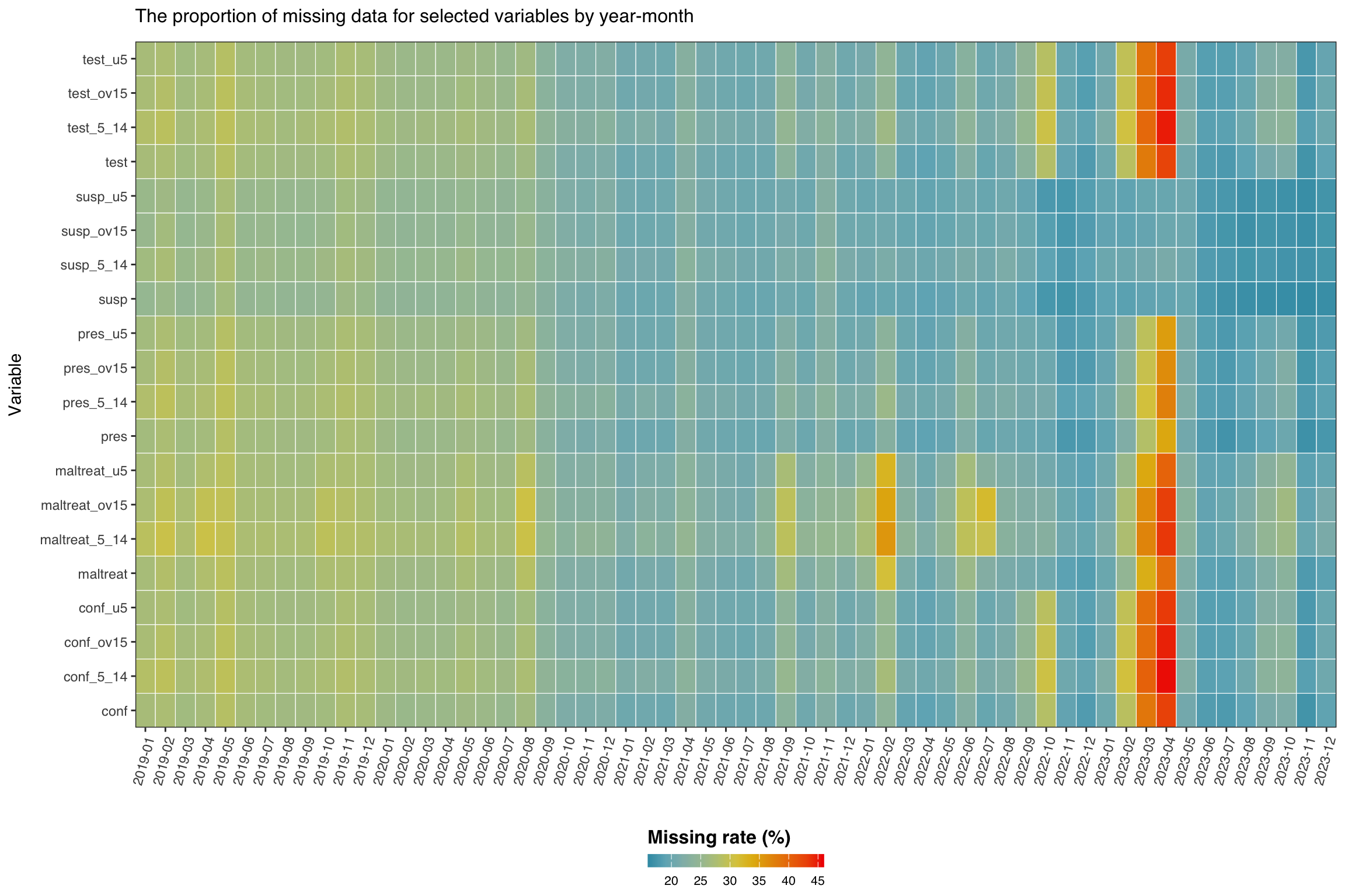
In this step we check the missingness rate of all of our variables of interest across time. This analysis helps us understand temporal patterns in data availability and identify periods or variables with systematic missing data issues. The heatmap visualization provides an intuitive overview of data completeness across all malaria indicators for different age groups throughout the study period. The color intensity represents the percentage of missing values, allowing us to quickly identify problematic time periods or variables that may require special handling in subsequent analyses.
Initially, we want to check the following set of variables: malaria tests, suspected, presumed and confirmed cases and malaria treatments aggregated across all age groups, as well as the age-specific breakdowns.
Show the code
# get the variables of interest (aggregated and age-specific)
vars <- c(
  "test",        # aggregated malaria tests
  "test_u5",
  "test_5_14",
  "test_ov15",
  "susp",        # aggregated suspected cases
  "susp_u5",
  "susp_5_14",
  "susp_ov15",
  "pres",        # aggregated presumed cases
  "pres_u5",
  "pres_5_14",
  "pres_ov15",
  "conf",        # aggregated confirmed cases
  "conf_u5",
  "conf_5_14",
  "conf_ov15",
  "maltreat",    # aggregated treatments
  "maltreat_u5",
  "maltreat_5_14",
  "maltreat_ov15"
)

# calculate missing rates by date for each variable
missing_rate_date <- df_routine |>
  dplyr::group_by(date) |>
  dplyr::summarise(
    dplyr::across(
      dplyr::all_of(vars),
      ~ mean(is.na(.x)) * 100
    ),
    .groups = "drop"
  ) |>
  dplyr::arrange(date) |>
  tidyr::pivot_longer(
    cols = -ym,
    names_to = "variables",
    values_to = "missing_rate"
  )

# Option to control the color scale range for the heatmap
# If TRUE: color scale goes from 0-100% (full range of possible missing rates,
# even if actual data doesnt cover this range)
# If FALSE: color scale is limited to actual range of missingness in the data
# (e.g., if missing rates range from 20-70%, color scale only covers that range)
full_range <- FALSE

# Set fill scale limits based on full_range option
fill_limits <- if (full_range) {
  c(0, 100) # Use full 0-100% range for color scale
} else {
  # Use actual range of missing rates in the data for color scale
  fill_var_values <- missing_rate_date$missing_rate
  c(
    floor(min(fill_var_values, na.rm = TRUE)),
    ceiling(max(fill_var_values, na.rm = TRUE))
  )
}

# plot the missing range across variables
missing_plot_date <- ggplot2::ggplot(
  missing_rate_date,
  ggplot2::aes(
    y = variables,
    x = ym,
    fill = missing_rate
  )
) +
  ggplot2::geom_tile(colour = "white", linewidth = .2) +
  ggplot2::scale_fill_gradientn(
    colours = wesanderson::wes_palette(
      "Zissou1",
      100,
      type = "continuous"
    ),
    limits = fill_limits
  ) +
  ggplot2::guides(
    fill = ggplot2::guide_colorbar(
      title.position = "top",
      nrow = 1,
      label.position = "bottom",
      direction = "horizontal",
      barheight = ggplot2::unit(0.3, "cm"),
      barwidth = ggplot2::unit(4, "cm"),
      ticks = TRUE,
      draw.ulim = TRUE,
      draw.llim = TRUE
    )
  ) +

  ggplot2::scale_x_discrete(expand = c(0, 0)) +
  ggplot2::scale_y_discrete(expand = c(0, 0)) +
  ggplot2::theme_bw() +
  ggplot2::theme(
    legend.title = ggplot2::element_text(
      size = 12,
      face = "bold",
      family = "sans"
    ),
    legend.position = "bottom",
    legend.direction = "horizontal",
    legend.box = "horizontal",
    legend.box.just = "center",
    legend.margin = ggplot2::margin(t = 0, unit = "cm"),
    legend.text = ggplot2::element_text(
      size = 8,
      family = "sans"
    ),
    axis.title.x = ggplot2::element_text(
      margin = ggplot2::margin(t = 5, unit = "pt")
    ),
    axis.title.y = ggplot2::element_text(
      margin = ggplot2::margin(r = 10, unit = "pt")
    ),
    axis.text.x = ggplot2::element_text(
      angle = 75,
      hjust = 1,
      family = "sans"
    ),
    axis.text = ggplot2::element_text(family = "sans"),
    axis.title = ggplot2::element_text(family = "sans"),
    plot.title = ggtext::element_markdown(
      size = 12,
      family = "sans",
      margin = ggplot2::margin(b = 10)
    ),
    strip.text = ggplot2::element_text(
      family = "sans",
      face = "bold"
    ),
    panel.grid.minor = ggplot2::element_blank(),
    panel.grid.major = ggplot2::element_blank(),
    panel.background = ggplot2::element_blank(),
    strip.background = ggplot2::element_rect(fill = "grey90")
  ) +
  ggplot2::labs(
    fill = "Missing rate (%)",
    y = "Variable",
    x = "",
    title = "The proportion of missing data for selected variables by year-month"
  )

# display the plot
missing_plot_date

# save plot
ggplot2::ggsave(
  plot = missing_plot_date,
  here::here("03_output/3a_figures/sle_many_vars_missing_plot_date.png"),
  width = 12,
  height = 7,
  dpi = 300
)
NoteOutput
To adapt the code:
Lines 2-23: Update the
varsvector to match your dataset’s variable names. For a different country/dataset, modify variable names to reflect your indicators (e.g., for Ghana you might havecases_u5,tests_5_14, etc.).Line 25: Replace
df_routinewith your dataset name if different.Line 37: Set
full_range <- TRUEif you want the color scale to always span 0-100% for consistent comparison across datasets/time periods. Setfull_range <- FALSEto optimize the color scale to your actual data range for better visual contrast within the observed missingness patterns.
TipUsing the sntutils Package
You can also reproduce this exact plot using the sntutils package, which provides additional features and customization options:
sntutils::reporting_rate_plot(
 data = df_routine,          # the dataset to use
 vars_of_interest = vars,    # a vector of vars to check
 x_var = "ym",               # the year-month var for the x axis
 use_reprate = FALSE,        # FALSE for missing rate, TRUE for reporting rate
 full_range = FALSE,         # use actual data range for fill
 target_language = "en"      # the language for plot labels
)
The sntutils::reporting_rate_plot() function includes additional parameters, such as specifying the language for plot labels and saving the output. See the sntutils documentation for more details.
Several indicators show consistent missingness across time. Between mid-2022 and early 2023, missingness sharply increased for several indicators, with test, maltreat, and conf reaching rates above 45%.
Step 2.2: Check Missingness Over Time and Administrative Level
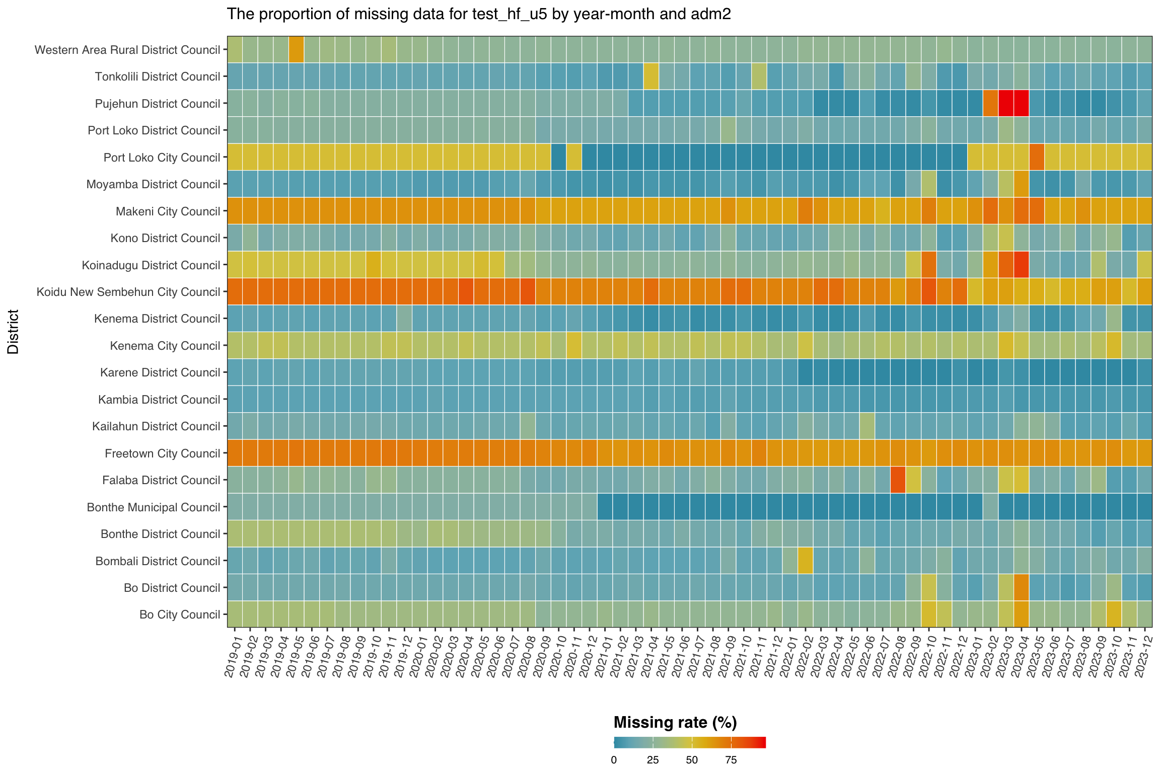
In this step, we focus on a single indicator, malaria testing for under 5’s at the health facility level (test_hf_u5), to examine how missingness varies over time across districts (admin2 level). This allows us to identify subnational areas with consistently poor reporting and spot time periods where data availability dropped sharply.
Although the data is available at the health facility level—the most granular reporting unit—it is still important to assess missingness at higher administrative levels. This broader view becomes especially useful when facility-level data are sparse. In such cases, we may use fallback imputation strategies that draw on patterns from neighbouring facilities within the same district.
Show the code
# calculate missing rates by year-month and adm2 for each variable
missing_rate_adm2 <- df_routine |>
  dplyr::group_by(ym, adm2) |>
  dplyr::summarise(
    missing_rate = mean(is.na(test_hf_u5)) * 100,
    .groups = "drop"
  )

# Option to control the color scale range for the heatmap
# If TRUE: color scale goes from 0-100% (full range of possible missing rates,
# even if actual data doesnt cover this range)
# If FALSE: color scale is limited to actual range of missingness in the data
# (e.g., if missing rates range from 20-70%, color scale only covers that range)
full_range <- FALSE

# Set fill scale limits based on full_range option
fill_limits <- if (full_range) {
  c(0, 100) # Use full 0-100% range for color scale
} else {
  # Use actual range of missing rates in the data for color scale
  fill_var_values <- missing_rate_adm2$missing_rate
  c(
    floor(min(fill_var_values, na.rm = TRUE)),
    ceiling(max(fill_var_values, na.rm = TRUE))
  )
}

# plot the missing range across location
missing_plot_adm2 <- ggplot2::ggplot(
  missing_rate_adm2,
  ggplot2::aes(
    y = adm2,
    x = ym,
    fill = missing_rate
  )
) +
  ggplot2::geom_tile(colour = "white", linewidth = .2) +
  ggplot2::scale_fill_gradientn(
    colours = wesanderson::wes_palette(
      "Zissou1",
      100,
      type = "continuous"
    ),
    limits = fill_limits
  ) +
  ggplot2::guides(
    fill = ggplot2::guide_colorbar(
      title.position = "top",
      nrow = 1,
      label.position = "bottom",
      direction = "horizontal",
      barheight = ggplot2::unit(0.3, "cm"),
      barwidth = ggplot2::unit(4, "cm"),
      ticks = TRUE,
      draw.ulim = TRUE,
      draw.llim = TRUE
    )
  ) +

  ggplot2::scale_x_discrete(expand = c(0, 0)) +
  ggplot2::scale_y_discrete(expand = c(0, 0)) +
  ggplot2::theme_bw() +
  ggplot2::theme(
    legend.title = ggplot2::element_text(
      size = 12,
      face = "bold",
      family = "sans"
    ),
    legend.position = "bottom",
    legend.direction = "horizontal",
    legend.box = "horizontal",
    legend.box.just = "center",
    legend.margin = ggplot2::margin(t = 0, unit = "cm"),
    legend.text = ggplot2::element_text(
      size = 8,
      family = "sans"
    ),
    axis.title.x = ggplot2::element_text(
      margin = ggplot2::margin(t = 5, unit = "pt")
    ),
    axis.title.y = ggplot2::element_text(
      margin = ggplot2::margin(r = 10, unit = "pt")
    ),
    axis.text.x = ggplot2::element_text(
      angle = 75,
      hjust = 1,
      family = "sans"
    ),
    axis.text = ggplot2::element_text(family = "sans"),
    axis.title = ggplot2::element_text(family = "sans"),
    plot.title = ggtext::element_markdown(
      size = 12,
      family = "sans",
      margin = ggplot2::margin(b = 10)
    ),
    strip.text = ggplot2::element_text(
      family = "sans",
      face = "bold"
    ),
    panel.grid.minor = ggplot2::element_blank(),
    panel.grid.major = ggplot2::element_blank(),
    panel.background = ggplot2::element_blank(),
    strip.background = ggplot2::element_rect(fill = "grey90")
  ) +
  ggplot2::labs(
    fill = "Missing rate (%)",
    y = "District",
    x = "",
    title = "The proportion of missing data for test_hf_u5 by year-month and adm2"
  )

# display the plot
missing_plot_adm2

# save plot
ggplot2::ggsave(
  plot = missing_plot_adm2,
  here::here("03_output/3a_figures/sle_test_missing_plot_adm2.png"),
  width = 12,
  height = 7,
  dpi = 300
)
NoteOutput
To adapt the code:
Line 1: Replace
df_routinewith your dataset name if different.Lines 5: Update the variable name (
test_hf_u5) to match your dataset’s variable name of interest.Line 13: Set
full_range <- TRUEif you want the color scale to always span 0-100% for consistent comparison across datasets/time periods. Setfull_range <- FALSEto optimize the color scale to your actual data range for better visual contrast within the observed missingness patterns.
TipUsing the sntutils Package
You can also reproduce this exact plot using the sntutils package.
sntutils::reporting_rate_plot(
 data = df_routine,              # the dataset to use
 vars_of_interest = "test_hf_u5",      # the var to check
 x_var = "ym",                   # the year-month var for the x axis
 y_var = "adm2",                 # the location var for the y axis
 y_axis_label = "District",      # Specify y axis lable (more readable)
 use_reprate = FALSE,            # FALSE for missing rate, TRUE for reporting rate
 full_range = FALSE,             # use actual data range for fill
 target_language = "en"          # the language for plot labels
)
Missing data for test_hf_u5 varies by district and over time. Freetown City Council, Port Loko City Council, Koidu New Sembehun Council, and Makeni City show consistently high missingness, especially from 2019 to mid-2021. Many districts also show increased missingness around mid to late 2022, suggesting a broader reporting issue. In contrast, districts like Falaba and Bonthe Municipal have lower and more stable missing rates. These patterns confirm that test_hf_u5 varies by both time and location.
This suggests that missingness in test_hf_u5 is likely Missing At Random (MAR), as it depends on observable factors such as district and reporting period. In such cases, stratified imputation is appropriate. The district (adm2) level can also serve as a fallback unit for imputation, particularly when individual facility data are sparse, by borrowing strength from neighbouring facilities within the same district.
Step 2.3: Check Missingness by Health Facility Type and Age Groups
Beyond temporal and geographic patterns, missingness may also vary systematically by additional factors, such as health facility type and age groups. Many routine surveillance systems collect data that is already disaggregated by these factors (e.g., test_hf_u5 representing malaria tests conducted at health facilities for children under 5).
The first step in determining these patterns is to disaggregate such pre-aggregated data into a long format, creating separate columns for indicators, facility types, and age groups. This long format allows us to examine how missingness varies across these important stratification variables and identify systematic reporting gaps that may be related to facility capacity, service delivery models, or demographic-specific data collection challenges.
Show the code
# define core indicators to retain during disaggregation
core_indicators <- c(
  "adm0",
  "adm1",
  "adm2",
  "adm3",
  "adm2",
  "hf",
  "hf_uid",
  "year",
  "month",
  "ym",
  "date"
)

# select core indicators and disaggregated variables
df_routine_disagg <- df_routine |>
  dplyr::select(
    dplyr::any_of(core_indicators),
    dplyr::matches("_(com|hf)_(u5|5_14|ov15)$")
  )

# transform to long format with separate facility type and age group columns
df_routine_disagg_long <- df_routine_disagg |>
  dplyr::select(-maladm_hf_u5) |> # drop maladm
  tidyr::pivot_longer(
    cols = dplyr::matches("_(com|hf)_(u5|5_14|ov15)$"),
    names_to = c("indicator", "facility_type", "age_group"),
    names_pattern = "(.+)_(com|hf)_(u5|5_14|ov15)$",
    values_to = "value"
  ) |>
  # relable factors
  dplyr::mutate(
    age_group = factor(
      age_group,
      levels = c("u5", "5_14", "ov15"),
      labels = c("Under 5", "5 to 15", "Over 15")
    ),
    facility_type = factor(
      facility_type,
      levels = c("hf", "com"),
      labels = c("Health Facility", "Community")
    )
  )

# preview the disaggregated data structure
head(df_routine_disagg_long)To adapt the code:
- Lines 2-6: Update the
core_indicatorsvector to match your dataset’s administrative and temporal variable names. - Line 9: Replace
df_routinewith your dataset name if different. - Lines 11 and 17: Modify the regex pattern
"_(com|hf)_(u5|5_14|ov15)$"to match your facility type and age group naming conventions (e.g., if your data uses different facility codes or age categories).
Now that we have disaggregated the data, we can examine how missingness varies across all indicators by facility type and age group. This check helps identify systematic patterns in data availability that may be related to service delivery models, facility capacity, or demographic-specific reporting challenges.
Show the code
# prepare data for stacked bar chart with both age group and facility type
missing_present_data_facility <- df_routine_disagg_long |>
  dplyr::group_by(indicator, age_group, facility_type) |>
  dplyr::summarise(
    total_records = dplyr::n(),
    missing_count = sum(is.na(value)),
    present_count = sum(!is.na(value)),
    missing_pct = round(missing_count / total_records * 100, 2),
    present_pct = round(present_count / total_records * 100, 2),
    .groups = "drop"
  ) |>
  tidyr::pivot_longer(
    cols = c(missing_pct, present_pct),
    names_to = "status",
    values_to = "percentage",
    names_pattern = "(.+)_pct"
  ) |>
  dplyr::mutate(
    status = factor(
      status,
      levels = c("missing", "present"),
      labels = c("Missing", "Present")
    )
  )

# create stacked bar plot faceted by age group and facility type
age_facility_miss_plot <- missing_present_data_facility |>
  ggplot2::ggplot(ggplot2::aes(
    x = percentage,
    y = factor(age_group, levels = rev(levels(factor(age_group)))),
    fill = status
  )) +
  ggplot2::geom_col(alpha = 0.8) +
  ggplot2::facet_grid(indicator ~ facility_type) +
  ggplot2::scale_fill_viridis_d(
    option = "D",
    begin = 0.2,
    end = 0.5,
    breaks = c("Present", "Missing")
  ) +
  ggplot2::guides(
    fill = ggplot2::guide_legend(
      title.position = "top",
      title.hjust = 0,
      label.position = "bottom"
    )
  ) +
  ggplot2::labs(
    title = "Missing vs Present Data by Indicator, Age Group, and Facility Type",
    x = "\nPercentage (%)",
    y = "Age Group (years)\n",
    fill = "Data Status"
  ) +
  ggplot2::scale_x_continuous(expand = c(0, 0)) +
  ggplot2::scale_y_discrete(expand = c(0, 0)) +
  ggplot2::theme_minimal() +
  ggplot2::theme(
    legend.position = "bottom",
    legend.direction = "horizontal",
    legend.justification = "left",
    legend.box.just = "left",
    axis.text.y = ggplot2::element_text(size = 8),
    strip.text = ggplot2::element_text(
      family = "sans",
      face = "bold"
    ),
    panel.grid.minor = ggplot2::element_blank(),
    panel.grid.major = ggplot2::element_blank(),
    panel.background = ggplot2::element_blank(),
    panel.border = ggplot2::element_rect(
      colour = "black",
      fill = NA,
      size = .7
    ),
    panel.spacing.x = ggplot2::unit(0.5, "cm"),
    plot.margin = ggplot2::margin(10, 20, 10, 10)
  )

# display the plot
age_facility_miss_plot

# save plot
ggplot2::ggsave(
  plot = age_facility_miss_plot,
  here::here("03_output/3a_figures/sle_test_facility_age_missing_plot.png"),
  width = 12,
  height = 7,
  dpi = 300
)
NoteOutput
-1.png)
To adapt the code:
- Line 2: Replace
df_routine_disagg_longwith your disaggregated dataset name if different. - Lines 13-20: Update the age group factor levels and labels to match your data structure and preferred display names.
- Lines 18-22: Modify facility type factor levels and labels according to your facility classification system.
The above visualization shows substantial differences in missingness patterns between facility types, with community-level facilities showing considerably higher missing rates, around 70% on average. This pattern is consistent across indicators and age groups. Notably, within community facilities, under-five data is more frequently reported than data for older age groups, a pattern observed across key indicators. These trends point to systematic differences in data collection and reporting capacity between facility types.
Step 2.4: Visualizing Structural Zeros and Logical Relationships
Before classifying missing values, we visualize the relationships between related indicators. This plot highlights likely structural zeros (e.g. no testing with missing confirmation), possible structural zeros (e.g. confirmed cases equal to zero with missing test values), and logical inconsistencies (e.g. confirmed cases recorded but testing data missing). These patterns reflect the clinical care pathway and help identify where values can be logically inferred, structurally imputed as zero, or require statistical methods.
Specifically:
- Test = 0, conf missing: Likely legitimate zero (no testing = confirmation not possible).
- Conf = 0, test missing: Possibly legitimate zero (no confirmed cases suggests no positives, but testing may have occurred).
- Conf > 0, test missing Logical inconsistency (confirmed cases imply testing occurred, value should be imputed).
- Test > 0, conf missing: Possibly legitimate zero (testing occurred but no positive cases; confirmation may be legitimately zero or missing).
Note: Below, we use the naniar package to explore missingness. Unlike geom_point(), which silently drops missing values, geom_miss_point() shows where one or both variables are missing by shifting them to plot margins. This makes it easier to detect structural zeros, reporting gaps, and logical inconsistencies.
Show the code
# transform data to wide format to examine relationships between indicators
df_wide <- df_routine_disagg_long |>
  dplyr::select(
    dplyr::any_of(core_indicators),
    facility_type,
    age_group,
    indicator,
    value
  ) |>
  tidyr::pivot_wider(
    names_from = indicator,
    values_from = value
  )

# calculate comprehensive missing counts for subtitle
n_test_missing_conf_zero <- df_wide |>
  dplyr::filter(conf == 0, is.na(test)) |>
  nrow()

n_conf_missing_test_zero <- df_wide |>
  dplyr::filter(test == 0, is.na(conf)) |>
  nrow()

n_test_na_conf_positive <- df_wide |>
  dplyr::filter(is.na(test), conf > 0) |>
  nrow()

n_conf_na_test_positive <- df_wide |>
  dplyr::filter(is.na(conf), test > 0) |>
  nrow()

# create comprehensive subtitle with all missing count scenarios
subtitle_text <- paste0(
  "N = ",
  scales::comma(n_test_missing_conf_zero),
  " where conf = 0 but test is missing (legitimate zero); \n",
  "N = ",
  scales::comma(n_conf_missing_test_zero),
  " where test = 0 but conf is missing (legitimate zero); \n",
  "N = ",
  scales::comma(n_test_na_conf_positive),
  " where test is missing but conf > 0 (logical inconsistency); \n",
  "N = ",
  scales::comma(n_conf_na_test_positive),
  " where conf is missing but test > 0 (possible legitimate zero)"
)

# create scatter plot showing relationship between test and confirmed counts
structural_zeros_plot <- ggplot2::ggplot(
  data = df_wide,
  mapping = ggplot2::aes(x = test, y = conf)
) +
  naniar::geom_miss_point() +
  ggplot2::geom_vline(
    xintercept = 0,
    linetype = "dashed",
    color = "grey40",
    linewidth = 0.2
  ) +
  ggplot2::geom_hline(
    yintercept = 0,
    linetype = "dashed",
    color = "grey40",
    linewidth = 0.2
  ) +
  ggplot2::scale_x_continuous(
    labels = scales::comma_format()
  ) +
  ggplot2::scale_y_continuous(
    labels = scales::comma_format()
  ) +
  ggplot2::scale_color_viridis_d(
    option = "D",
    begin = 0.2,
    end = 0.5,
    breaks = c("Not Missing", "Missing"),
    labels = c("Present", "Missing")
  ) +
  ggplot2::guides(
    color = ggplot2::guide_legend(
      title.position = "top",
      title.hjust = 0,
      override.aes = list(
        size = 5
      ),
      label.position = "bottom"
    )
  ) +
  ggplot2::labs(
    title = "Structural Zeros: Testing vs Confirmation",
    subtitle = subtitle_text,
    x = "\nTests Conducted",
    y = "Cases Confirmed\n",
    color = "Data Status"
  ) +
  ggplot2::theme_minimal() +
  ggplot2::theme(
    legend.position = "bottom",
    legend.direction = "horizontal",
    legend.justification = "left",
    legend.box.just = "left",
    axis.text.y = ggplot2::element_text(size = 8),
    strip.text = ggplot2::element_text(
      family = "sans",
      face = "bold"
    ),
    panel.border = ggplot2::element_rect(
      colour = "black",
      fill = NA,
      size = .7
    ),
    panel.spacing.x = ggplot2::unit(0.5, "cm"),
    plot.margin = ggplot2::margin(10, 20, 10, 10),
    plot.subtitle = ggplot2::element_text(size = 9, color = "grey30")
  )


# display the plot
structural_zeros_plot

# save plot
ggplot2::ggsave(
  plot = structural_zeros_plot,
  here::here("03_output/3a_figures/sle_test_conf_check_zeros_plot.png"),
  width = 12,
  height = 7,
  dpi = 300
)
NoteOutput
-1.png)
To adapt the code:
Key variables: Update the variable names (
test,maltreat) to match your dataset’s variable names of interest.Lines 2-10: Update the
core_indicatorsand column selection to match your dataset structure.Lines 15-20: Modify the
pivot_wider()transformation to include the specific indicators you want to examine for structural relationships.Lines 22-28: Update facility type factor levels and labels to match your classification system.
Lines 31-32: Change the x and y aesthetic mappings to examine different variable pairs (e.g.,
x = maltreat, y = confto examine treatment vs confirmation relationships).
The plot shows key patterns in missingness between malaria testing (test) and confirmation (conf) counts. The vertical dashed line marks zero tests; the horizontal dashed line marks zero confirmations. This visualization shows there were 1,769 instances where conf is missing but test > 0. These are likely structural zeros, where testing was done but no confirmed cases were recorded. In such cases, missing confirmation counts can reasonably be set to zero.
Step 3: Determining HF Active vs Non-Active Status and Inferring Zeros vs NA
Before applying any imputation method, it is essential to assess whether a missing value reflects a non-active health facility status (i.e. the facility was not reporting at the time), or whether it is a reporting omission (i.e. the facility was active but left a value blank). This distinction determines whether a missing value should be excluded, imputed as zero, or left as NA.
Step 3.1: HF Non-Active Status
Some missing values are not true gaps but reflect periods where the facility was not yet reporting or never reported that specific indicator. These reflect non-active health facility status and should not be imputed.
We use the following derived variables to detect non-active health facility status:
first_reporting_date: The first year-month in which a health facility (hf_uid) reported key indicators specified. Used to determine when the facility became active in routine reporting.never_reported_<indicator>: Logical flag indicating whether the facility never reported a non-missing value for a specific indicator during its reporting span. TRUE means it was never reported.reported_any: Logical flag indicating whether the facility reported any of the selected key indicators in a given year-month. Used to detect whether a form was likely submitted for that time point.
A facility-indicator-month is considered to have non-active HF status if any of the conditions in the table below are met.
| Condition | Interpretation | Action |
|---|---|---|
date < first_reporting_date
|
Facility was not active yet | 🚫 Not missing but expected |
never_reported_<indicator> == TRUE
|
Facility never used this indicator | 🚫 Not missing but expected |
reported_any == FALSE
|
Facility did not submit any data that month | 🚫 Not missing but expected. Full form likely missing – skip |
This filtering step will be helpful later in determining eligibility for imputation, ensuring that it is applied only to year-months when the facility was active and the indicator was expected to be used. Non-active HF status periods are excluded from all further imputation steps.
ImportantConsult with SNT Team
Some apparent gaps may be due to facilities not yet activated or not expected to report certain indicators. Confirm with the SNT team before deciding whether these values should be marked as ‘not applicable’ or considered missing.
Show the code
# define key columns of interest
key_indicator_cols <- c(
  "test_hf_u5",
  "susp_hf_u5",
  "pres_hf_u5",
  "conf_hf_u5",
  "maltreat_hf_u5"
)

# generate full grid of all hf_uid and date combinations
full_grid <- tidyr::expand_grid(
  hf_uid = unique(df_routine$hf_uid),
  date = seq(min(df_routine$date), max(df_routine$date), by = "month")
)

# left join with your routine data
df_routine_balanced <- full_grid |>
  dplyr::left_join(df_routine, by = c("hf_uid", "date"))

# create reporting pattern analysis
routine_reporting_elig <- df_routine_balanced |>
  dplyr::mutate(
    # count how many indicators were reported (non-NA)
    indicators_reported = dplyr::across(dplyr::all_of(key_indicator_cols)) |>
      (\(x) rowSums(!is.na(x)))(),

    # mark rows where any indicator was reported
    reported_any = indicators_reported > 0
  ) |>
  dplyr::group_by(hf_uid) |>
  dplyr::mutate(
    # cumulative max to track if the facility has ever reported by that month
    has_ever_reported = cummax(reported_any),

    # date when the facility first reported any indicator
    first_reporting_date = if (any(reported_any)) {
      min(date[reported_any], na.rm = TRUE)
    } else {
      as.Date(NA)
    },
    #  classify each facility-month as 'active_reporting',
    # 'active_not_reporting', or 'inactive'
    activity_status = dplyr::case_when(
      reported_any ~ "Active Reporting",
      !reported_any & has_ever_reported ~ "Active Facility — Not Reporting",
      !reported_any & !has_ever_reported ~ "Inactive Facility"
    ),
    activity_status = factor(
      activity_status,
      level = c("Active Reporting", "Active Facility — Not Reporting", "Inactive Facility")
    )
  ) |>
  dplyr::ungroup()

# facility activeness plot
facility_activeness <-
  routine_reporting_elig |>
  dplyr::filter(!is.na(first_reporting_date)) |>
  ggplot2::ggplot(
    ggplot2::aes(
      x = date,
      y = forcats::fct_reorder(hf_uid, first_reporting_date),
      fill = activity_status
    )
  ) +
  ggplot2::geom_tile(
    width = 31,
    height = 1
  ) +
  ggplot2::scale_fill_manual(
    values = c(
      "Active Reporting" = "#1b9e77",
      "Active Facility — Not Reporting" = "#e7298a",
      "Inactive Facility" = "#d9d9d9"
    ),
    na.value = "grey90",
    name = "Reported any key indicator"
  ) +
  ggplot2::scale_x_date(
    expand = c(0, 0),
    date_labels = "%b %Y",
    date_breaks = "3 months"
  ) +
  ggplot2::labs(
    x = " ",
    y = NULL,
    title = glue::glue(
      "Monthly reporting activity by health facility ",
      "(n={format(dplyr::n_distinct(routine_reporting_elig$hf_uid),
      big.mark = \",\")})"
    )
  ) +
  ggplot2::theme_minimal(base_family = "sans") +
  ggplot2::guides(
    fill = ggplot2::guide_legend(
      title.position = "top",
      label.position = "bottom",
      keywidth = grid::unit(4.5, "lines")
    )
  ) +
  ggplot2::theme(
    axis.text.y = ggplot2::element_blank(),
    # axis.ticks.y = ggplot2::element_blank(),
    axis.line = ggplot2::element_line(color = "black", linewidth = 0.5),
    axis.text.x = ggplot2::element_text(angle = 45, hjust = 1),
    legend.position = "bottom",
    legend.direction = "horizontal",
    legend.box = "vertical"
  )

# display the plot
facility_activeness

# save plot
ggplot2::ggsave(
  plot = facility_activeness,
  here::here("03_output/3a_figures/sle_facility_activeness.png"),
  width = 12,
  height = 7,
  dpi = 300
)
NoteOutput
-1.png)
To adapt the code:
- Lines 2-7: Replace
key_indicator_colsvalues with your specific indicator column names if different fromtest_hf_u5,susp_hf_u5,pres_hf_u5,conf_hf_u5,maltreat_hf_u5. - Line 9: Replace
df_routinewith your dataset name if different. - Line 10: Adjust the date sequence parameters to match your data’s date range and desired time intervals.
- Line 104: Replace with your facility identifier variable name if different from
hf_uid.
NoteNote on Row Expansion
To assess facility reporting patterns consistently, we expand the dataset to include every possible combination of hf_uid and month within the observed range. This ensures that both reporting and non-reporting months are represented. As a result, the number of rows increases from 102,360 (original reported months only) to 106,260, adding 3,900 non-active HF status months where facilities were present but did not report any key indicators.
Step 3.2: Zeros vs NA - Interpreting Gaps Within Active Reporting
After identifying non-active HF status in Step 3.1, the dataset now includes flags that help distinguish between reporting gaps and periods where the facility was likely not functional or not expected to report. These flags are used to conditionally exclude certain data points from imputation, without removing them from the dataset.
We focus now on interpreting missing values that occur during active reporting periods. These are time points where a facility was expected to report but left some fields blank. Such missingness can arise due to:
- A true zero (e.g. no cases that month), or
- A reporting omission (e.g. staff left the field blank or forgot to enter the value)
Treating all NAs as zeros can lead to underestimation. Conversely, imputing values when the facility was inactive or not reporting distorts the data. The goal is to impute selectively, only where appropriate.
We use the following table to guide imputation eligibility:
| Condition | Interpretation | Action |
|---|---|---|
date < first_reporting_date
|
Facility was not active yet |
🚫 Flag as Inactive. Exclude from imputation
|
never_reported_<indicator> == TRUE
|
Facility never used this indicator |
🚫 Flag as Inactive. Exclude from imputation
|
reported_any == FALSE
|
Facility did not submit any data that month |
🚫 Flag as Active Not Reporting. Exclude from imputation
|
reported_any == TRUE and value is NA
|
Likely omission for this indicator |
✅ Flag as Active Reporting. missing but expected
|
reported_any == TRUE and value is 0
|
Confirmed zero cases reported | ✅ Keep as is (no imputation needed) |
This structured approach helps ensure imputation is applied only to missing values during active reporting, avoided where missingness is structural, and sensitive to whether zeros are meaningful and observed.
Now we implement this logic to create imputation eligibility flags and examine the patterns:
Show the code
# create never_reported flags for specific indicators using key_indicator_cols
never_reported_flags <- routine_reporting_elig |>
  dplyr::group_by(hf_uid) |>
  dplyr::summarise(
    never_reported_indicator = all(is.na(test_hf_u5)),
    .groups = "drop"
  )

# join back to main dataset and create imputation eligibility for test_hf_u5
imputation_elig <- routine_reporting_elig |>
  dplyr::left_join(never_reported_flags, by = "hf_uid") |>
  dplyr::mutate(
    # create imputation eligibility flag for test_hf_u5
    imputation_status = dplyr::case_when(
      activity_status == "Inactive Facility" ~ "Inactive Facility",
      never_reported_indicator == TRUE ~ "Indicator Never Reported",
      activity_status == "Active Facility — Not Reporting" ~ "Active Facility — Not Reporting",
      activity_status == "Active Reporting" &
        is.na(test_hf_u5) ~
        "Missing but Expected",
      activity_status == "Active Reporting" &
        !is.na(test_hf_u5) ~
        "Reported (non-missing)",
      TRUE ~ "Unknown"
    ),
    imputation_status = factor(
      imputation_status,
      levels = c(
        "Reported (non-missing)",
        "Missing but Expected",
        "Active Facility — Not Reporting",
        "Indicator Never Reported",
        "Inactive Facility",
        "Unknown"
      )
    )
  )

# get counts for legend labels
eligibility_counts <- imputation_elig |>
  dplyr::count(imputation_status) |>
  dplyr::mutate(
    label_with_n = paste0(
      imputation_status,
      " (n=",
      format(n, big.mark = ","),
      ")"
    )
  )

# create named vector for labels
legend_labels <- setNames(
  eligibility_counts$label_with_n,
  eligibility_counts$imputation_status
)

# create visualization showing imputation eligibility patterns
test_patterns <- imputation_elig |>
  dplyr::filter(!is.na(first_reporting_date)) |>
  dplyr::select(hf_uid, date, first_reporting_date, imputation_status)

# create imputation eligibility heatmap
imputation_eligibility_plot <- test_patterns |>
  ggplot2::ggplot(
    ggplot2::aes(
      x = date,
      y = forcats::fct_reorder(hf_uid, first_reporting_date),
      fill = imputation_status
    )
  ) +
  ggplot2::geom_tile(
    width = 31,
    height = 1
  ) +
  ggplot2::scale_fill_manual(
    values = c(
      "Reported (non-missing)" = "#1b9e77",
      "Missing but Expected" = "#ffdd57",
      "Active Facility — Not Reporting" = "#e66101",
      "Indicator Never Reported" = "#762a83",
      "Inactive Facility" = "#d9d9d9",
      "Unknown" = "#4575b4"
    ),
    labels = legend_labels,
    na.value = "white",
    name = "Imputation Status"
  ) +
  ggplot2::scale_x_date(
    expand = c(0, 0),
    date_labels = "%b %Y",
    date_breaks = "3 months"
  ) +
  ggplot2::labs(
    x = " ",
    y = NULL,
    title = "Imputation eligibility patterns for test_hf_u5 by health facility",
    subtitle = glue::glue(
      "Analysis of {format(dplyr::n_distinct(test_",
      "patterns$hf_uid), big.mark = ',')} facilities ",
      "showing data availability and imputation eligibility"
    )
  ) +
  ggplot2::theme_minimal(base_family = "sans", base_size = 12) +
  ggplot2::guides(
    fill = ggplot2::guide_legend(
      title.position = "top",
      label.position = "bottom",
      keywidth = grid::unit(3, "lines"),
      nrow = 2
    )
  ) +
  ggplot2::theme(
    axis.text.y = ggplot2::element_blank(),
    axis.line = ggplot2::element_line(color = "black", linewidth = 0.5),
    axis.text.x = ggplot2::element_text(angle = 45, hjust = 1),
    legend.position = "bottom",
    legend.direction = "horizontal",
    legend.box = "vertical",
    plot.subtitle = ggplot2::element_text(size = 14, color = "gray50")
  )

# display the plot
imputation_eligibility_plot

# save plot
ggplot2::ggsave(
  plot = imputation_eligibility_plot,
  here::here(
    "03_output/3a_figures/sle_test_imputation_eligibility_plot.png"
  ),
  width = 12,
  height = 7,
  dpi = 300
)
NoteOutput
-1.png)
To adapt the code:
- Line 4: Replace
test_hf_u5with your indicator of interest for the never-reported analysis. - Lines 11-19: Update the
case_when()logic to use your specific indicator name instead oftest_hf_u5. - Lines 21-24: Modify the factor levels based on the categories relevant to your analysis.
- Lines 47-53: Customize the color palette for different eligibility statuses if desired.
We now have a clear basis for imputation. Of all facility-months, 77,699 had valid data and 2,271 were missing but expected. The rest were flagged as structurally absent: 2,885 were active but not reporting, 201 never reported the indicator, and 23,204 were inactive. This ensures imputation is limited to valid gaps during active reporting periods. In the subsequent section, we will use the imputation_status flag to conditionally impute the test_hf_u5 variable.
Step 4: Resolve Missing Data
Now that we have identified which observations are missing but expected, we resolve missing test_hf_u5 values using a two-stage approach:
Stage 1: Structural Imputation - Apply epidemiological logic to cases where missing values can be definitively inferred from the reporting sequence that we established earlier in our Imputation Decision Framework.
Stage 2: Moving Average Imputation - For the remaining missing values, we apply constrained moving average imputation to capture temporal trends as well as patterns by facility type, age group, and location. This method provides more robust estimates than simple techniques that ignore time and contextual structur
This sequential approach ensures that we first use the inherent logical relationships in malaria data (Stage 1: structural imputation), before applying time-aware methods that respect both clinical logic and observed reporting patterns.
Step 4.1: Structural Imputation Implementation (Stage 1)
Now we implement the clinical logic framework created in Apply Clinical Logic: Systematic Classification of Missing Values section. For each missing test_hf_u5 value, we systematically check for downstream evidence and classify the missingness:
Before applying any structural imputation, we must first identify the upstream and downstream variables that will inform the imputation of test_hf_u5.
Show the code
# Get Upstream and Downstream Variables for Malaria Pathway Indicators
#
# Determines upstream and downstream variables for a given malaria indicator
# based on the clinical care pathway. Structural imputation is only allowed
# for indicators that follow predictable relationships in the pathway.
#
# Assumes variable names match standard: 'susp', 'test', 'conf',
# 'maltreat', 'maladm', 'maldth'.
#
# @param var_to_impute Character. Variable name to analyze (e.g., "conf").
#   Do not include suffix here; suffix is appended separately if provided.
# @param malaria_pathway Character vector. Ordered indicator sequence.
# @param facility_type Character or NULL. Facility type. Used to restrict
#   imputation for admissions ('maladm'), which only apply to inpatient-
#   capable facilities. Examples include: "hospital", "referral", "inpatient",
#   "health_facility" or "tertiary". All other facility types
#   (e.g., "health_post", "clinic") are treated as outpatient-only.
# @param suffix Character or NULL. Optional suffix to append to variable names
#   in output (e.g., "_hf" to return "test_hf", "conf_hf").
#
# @return A list with:
# \describe{
#   \item{var_to_impute}{Indicator with suffix applied.}
#   \item{upstream_vars}{Indicators that logically precede it.}
#   \item{downstream_vars}{Indicators that logically follow it.}
#   \item{use_structural}{Logical. TRUE if structural imputation is allowed.}
# }
#
# @details
# Indicator usage in imputation logic depends on facility type.
# Admissions ('maladm') are only included at inpatient-capable facilities.
## +------------+-----------------+--------------------+-----------------------+
## | Indicator  | Facility Type   | Upstream Used      | Downstream Used       |
## +------------+-----------------+--------------------+-----------------------+
#  | susp       | All             | —                  | test, conf, maladm*,  |
#  |            |                 |                    | maldth                |
#  | test       | All             | susp               | conf, maladm*, maldth |
#  | conf       | All             | susp, test         | maladm*, maldth       |
#  | maltreat   | All             | susp, test, conf   | maladm*, maldth       |
#  | maladm     | Inpatient only  | susp, test, conf   | maldth                |
#  | maladm     | Outpatient only | —                  | —                     |
#  | maldth     | All             | susp, test, conf,  |                       |
#  |            |                 | maladm*            | —                     |
## +------------+-----------------+--------------------+-----------------------+
# * Only used if facility is inpatient-capable
#
# @examples
# get_pathway_vars("test")
# get_pathway_vars("conf", suffix = "_hf")
# get_pathway_vars("maltreat")
# get_pathway_vars("maladm", facility_type = "hospital")
# get_pathway_vars("maladm", facility_type = "health_post")
#
# @export
get_pathway_vars <- function(
  var_to_impute,
  malaria_pathway = c("susp", "test", "conf", "maltreat", "maladm", "maldth"),
  facility_type = NULL,
  suffix = NULL
) {
  append_suffix <- function(x) {
    if (length(x) == 0) {
      character()
    } else if (is.null(suffix)) {
      x
    } else {
      paste0(x, suffix)
    }
  }

  inpatient_types <- c("hospital", "referral", "inpatient", "tertiary")

  if (var_to_impute == "maladm") {
    is_inpatient <- !is.null(facility_type) &&
      tolower(facility_type) %in% tolower(inpatient_types)

    if (!is_inpatient) {
      cli::cli_h1("Malaria Pathway Summary")
      cli::cli_alert_info(
        "Imputing for {.field {append_suffix(var_to_impute)}}"
      )
      cli::cli_alert_danger(
        "Admissions not applicable at outpatient facilities (e.g., health post)."
      )
      cli::cli_alert_warning("Structural imputation excluded")
      cli::cli_alert_success("Upstream: None")
      cli::cli_alert_success("Downstream: None")

      return(list(
        var_to_impute = append_suffix(var_to_impute),
        upstream_vars = character(),
        downstream_vars = character(),
        use_structural = FALSE
      ))
    }
  }

  is_inpatient <- !is.null(facility_type) &&
    tolower(facility_type) %in% tolower(inpatient_types)

  non_linear <- character()
  if (var_to_impute != "maltreat") {
    non_linear <- c(non_linear, "maltreat")
  }
  if (!is_inpatient) {
    non_linear <- c(non_linear, "maladm")
  }

  linear_path <- malaria_pathway[!malaria_pathway %in% non_linear]
  pos <- match(var_to_impute, linear_path)

  upstream_vars <- if (is.na(pos) || pos <= 1) {
    character()
  } else {
    linear_path[1:(pos - 1)]
  }

  downstream_vars <- if (is.na(pos) || pos >= length(linear_path)) {
    character()
  } else {
    linear_path[(pos + 1):length(linear_path)]
  }

  upstream_str <- if (length(upstream_vars) == 0) {
    "None"
  } else {
    paste(append_suffix(upstream_vars), collapse = ", ")
  }
  downstream_str <- if (length(downstream_vars) == 0) {
    "None"
  } else {
    paste(append_suffix(downstream_vars), collapse = ", ")
  }

  cli::cli_h1("Malaria Pathway Summary")
  cli::cli_alert_info("Imputing for {.field {append_suffix(var_to_impute)}}")
  cli::cli_alert_success("Upstream: {.field {upstream_str}}")
  cli::cli_alert_success("Downstream: {.field {downstream_str}}")

  if (
    var_to_impute != "maladm" &&
      "maladm" %in% malaria_pathway &&
      !is_inpatient
  ) {
    cli::cli_alert_info(
      paste0(
        "Note: {.val ",
        append_suffix("maladm"),
        "} excluded from dependency logic due to outpatient facility."
      )
    )
  }

  if (
    var_to_impute != "maltreat" &&
      "maltreat" %in% malaria_pathway
  ) {
    cli::cli_alert_info(
      paste0(
        "Note: {.val ",
        append_suffix("maltreat"),
        "} excluded from dependency logic due to presumptive treatment."
      )
    )
  }

  cli::cat_line()

  return(list(
    var_to_impute = append_suffix(var_to_impute),
    upstream_vars = append_suffix(upstream_vars),
    downstream_vars = append_suffix(downstream_vars),
    use_structural = TRUE
  ))
}

# get upstream and downstream indicators
ud_test_hf <- get_pathway_vars(
  var_to_impute = "test",
  malaria_pathway = c("susp", "test", "conf", "maltreat", "maladm", "maldth"),
  suffix = "_hf_u5",
facility_type = "hospital"To adapt the code:
- Line 24: Replace
var_to_imputewith the base name of your variable (e.g.conf). - Line 25: Replace
malaria_pathwaywith your clinical pathway if different. - Line 26: Replace
suffixwith the string appended to each indicator (e.g._hf_u5), matching your column naming convention based on the disaggregation used in your data (e.g._male_u5,_com_ov5). - Line 27: Replace
facility_typebased on the type of facility (e.g.hospital,health_post).
Based on the clinical care pathway, we have established the relevant indicators for test_hf_u5. The upstream indicator is susp_hf_u5, while the downstream indicators are conf_hf_u5, maladm_hf_u5, and maldth_hf_u5. The indicator maltreat_hf_u5 is excluded from the dependency logic due to the possibility of presumptive treatment.
In the following step, these indicators guide the imputation logic
- Minimum constraint imputation: Downstream indicators > 0 → establish minimum bound (
test_hf_u5≥ max downstream value) and apply statistical imputation with constraint - Structural zero: No suspects and all downstream = 0/missing → impute
test_hf_u5= 0 - Defer to statistical methods: Suspects exist but no downstream evidence → flag for moving average without constraints
Important: When downstream indicators exist, they represent the minimum value that test_hf_u5 must have, not the exact value. For example, if maldth_hf_u5 = 2, then test_hf_u5 ≥ 2. This allows for statistical imputation while respecting logical constraints.
This implementation processes the data systematically, creating a comprehensive record of imputation decisions and sources.
The output table below summarizes the structural classification, downstream evidence, and imputation source for each record flagged as eligible.
Show the code
# extract dynamic components from the pathway definition
upstream_vars <- ud_test_hf$upstream_vars
downstream_vars <- ud_test_hf$downstream_vars
use_structural <- ud_test_hf$use_structural
var_to_impute <- rlang::sym(ud_test_hf$var_to_impute)

imputation_elig_str <- imputation_elig |>
  dplyr::mutate(
    # binary column determining whether var_to_impute requires imputation
    to_impute = coalesce(imputation_status == "Missing but Expected", FALSE),
    # check the existence of positive downstream
    has_positive_upstream = if (length(upstream_vars) == 0L) {
      FALSE
    } else {
      rowSums(
        dplyr::across(
          dplyr::any_of(upstream_vars),
          ~ (!is.na(.x) & .x > 0) + 0L
        ),
        na.rm = TRUE
      ) >
        0
    },
    # check the existence of positive upstream
    has_positive_downstream = if (length(downstream_vars) == 0L) {
      FALSE
    } else {
      rowSums(
        dplyr::across(
          dplyr::any_of(downstream_vars),
          ~ (!is.na(.x) & .x > 0) + 0L
        ),
        na.rm = TRUE
      ) >
        0
    },
  ) |>
  # classify structural pattern based on logic
  dplyr::mutate(
    structural_classification = dplyr::case_when(
      !is.na({{ var_to_impute }}) ~ "Value observed",
      to_impute &
        is.na({{ var_to_impute }}) &
        !has_positive_upstream &
        !has_positive_downstream ~
        "No pathway evidence reported",
      to_impute & is.na({{ var_to_impute }}) & has_positive_downstream ~
        "Positive downstream indicators reported",
      to_impute &
        is.na({{ var_to_impute }}) &
        has_positive_upstream &
        !has_positive_downstream ~
        "Positive upstream reported, no downstream evidence",
      !to_impute ~ "Not eligible for imputation",
      TRUE ~ "Pattern unclear"
    )
  ) |>
  # compute rowwise max from downstream indicators
  dplyr::mutate(
    max_downstream = if (length(downstream_vars) == 0L) {
      NA_real_
    } else {
      raw <- do.call(
        pmax,
        c(
          as.list(dplyr::select(
            cur_data_all(),
            dplyr::any_of(downstream_vars)
          )),
          na.rm = TRUE
        )
      )
      raw[is.infinite(raw) & raw < 0] <- NA_real_
      raw
    }
  ) |>
  dplyr::ungroup() |>

  # apply minimum constraint where relevant
  dplyr::mutate(
    minimum_constraint = dplyr::case_when(
      has_positive_downstream & is.na({{ var_to_impute }}) ~ max_downstream,
      TRUE ~ NA_real_
    )
  ) |>
  # pre-compute matching downstream variable for cleaner logic
  dplyr::mutate(
    matching_downstream = {
      matches <- downstream_vars[downstream_vars == max_downstream]
      if (length(matches) == 1) {
        matches
      } else {
        "Statistical imputation (constrained)"
      }
    },
    imputation_source = dplyr::case_when(
      !is.na({{ var_to_impute }}) ~ "Original value",
      structural_classification == "No pathway evidence reported" ~
        "Set to zero (imputation)",
      structural_classification == "Positive downstream indicators reported" ~
        matching_downstream,
      structural_classification == "Not eligible for imputation" ~
        "None - no imputation",
      TRUE ~ "Statistical imputation"
    )
  ) |>
  dplyr::select(-matching_downstream) |>
  # flag unclear or uncertain cases
  dplyr::mutate(
    needs_review = structural_classification %in%
      c(
        "Positive downstream indicators reported",
        "Positive upstream reported, no downstream evidence",
        "Pattern unclear"
      )
  )

# impute legitimate zero rows to 0
imputation_elig_str <- imputation_elig_str |>
  dplyr::mutate(
    "{var_to_impute}_structural" := dplyr::if_else(
      imputation_source == "Set to zero (imputation)",
      0,
      {{ var_to_impute }}
    )
  )

# display classification summary
imputation_elig_str |>
  dplyr::filter(structural_classification != "Not eligible for imputation") |>
  dplyr::count(structural_classification, imputation_source, sort = TRUE) |>
  dplyr::mutate(Count = scales::comma(n)) |>
  dplyr::select(
    `Structural Classification` = structural_classification,
    `Imputation Source` = imputation_source,
    Count
  ) |>
  knitr::kable(
    caption = glue::glue(
      "Summary of Structural Classifications and Sources Used ",
      "in Imputing Missing `{var_to_impute}` Values"
    )
)To adapt the code:
- Lines 2-4: Modify the
upstream_varsanddownstream_varsvectors to include the relevant indicators in your malaria care pathway. - Lines 22-37: Adjust the classification logic in
structural_classificationif you have different dependency rules. - Lines 55-70: The structural imputation implementation creates comprehensive imputation tracking and applies legitimate zero rules.
In total, 13,884 missing test_hf_u5 values were classified: 11,514 rows with reported suspected cases but no downstream outcomes, requiring statistical imputation; 2,328 rows eligible for minimum-constrained imputation using the available as upstream input; and 42 rows flagged as structural zeros with no evidence of testing, which were set to zero.
The following table shows sample records from each structural classification where testing occurred but values were missing, along with the downstream source used for imputation:
ImportantValidate with SNT Team
Before proceeding to statistical imputation, review the structural imputation results with the SNT team. Are imputed values consistent with clinical logic and local program knowledge? This review helps catch incorrect assumptions (e.g., test counts below confirmed cases).
Step 4.2: Implement Constrained Moving Average Imputation (Stage 1)
For missing test_hf_u5 values not addressed through structural imputation, we apply constrained moving average imputation. This method preserves epidemiological consistency by ensuring that imputed testing values do not fall below observed downstream indicators (e.g. confirmed cases or malaria deaths), while also capturing temporal trends.
This step implements a hierarchical rolling mean strategy to account for variability in data availability across facilities:
Primary grouping: A 3-period right-aligned moving average is calculated at the health facility level (
hf_uid). This captures individual facility trends over time for a specific hf_type and age_group.Fallback grouping: Where the facility-level window is missing or insufficient, a secondary 3-period moving average is calculated at the adm2 level. This provides a spatial fallback for sparse or irregularly reporting facilities.
Constraint logic: Each candidate imputed value is constrained to be no less than a predefined minimum_constraint, typically the maximum of downstream idnicators like conf or maldth values for that record. This constraint ensures that the imputed number of tests cannot be lower than the number of confirmed cases or malaria deaths, preserving indicator consistency across the care pathway.
Imputation proceeds as follows:
- If the original value is non-missing, it is retained.
- If missing and structural zeros are known, they are used.
- If missing and not structural, we impute using the facility-level moving average (if available).
- If that is also missing, we use the fallback from adm2-level grouping.
- If all else fails, the value is set to the minimum_constraint.
This structured imputation logic ensures transparency and reproducibility in how missing test_hf_u5 values are filled, with all decisions traceable by facility and time.
Show the code
# create variable names for injection and symbols for cleaner injection
var_roll_primary <- paste0(var_to_impute, "_roll_primary") |> rlang::sym()
var_fallback <- paste0(var_to_impute, "_fallback") |> rlang::sym()
var_original <- paste0(var_to_impute, "_original") |> rlang::sym()
var_imp_stat <- paste0(var_to_impute, "_imp_stat") |> rlang::sym()
var_final <- paste0(var_to_impute, "_final") |> rlang::sym()
var_structural <- paste0(var_to_impute, "_structural") |> rlang::sym()
var_to_impute_sym <- var_to_impute |> rlang::sym()
var_imputed_name <- paste0(var_to_impute, "_final_decision") |> rlang::sym()

# constrained moving average imputation
imputation_elig_stat <- imputation_elig_str |>
  dplyr::arrange(hf_uid, date) |>
  dplyr::mutate(
    !!var_roll_primary := zoo::rollmean(
      !!var_structural,
      k = 3,
      fill = NA,
      align = "right"
    ) |>
      round()
  ) |>
  dplyr::ungroup() |>
  # compute fallback (adm3-level) rolling means
  dplyr::group_by(adm2) |>
  dplyr::mutate(
    !!var_fallback := zoo::rollmean(
      !!var_structural,
      k = 3,
      fill = NA,
      align = "right"
    ) |>
      round()
  ) |>
  dplyr::ungroup() |>
  # impute using the available rolling mean + constraint
  dplyr::mutate(
    !!var_original := test,
    !!var_imp_stat := dplyr::case_when(
      !is.na(!!var_roll_primary) ~
        pmax(!!var_roll_primary, minimum_constraint, na.rm = TRUE),
      !is.na(!!var_fallback) ~
        pmax(!!var_fallback, minimum_constraint, na.rm = TRUE),
      TRUE ~ minimum_constraint
    ),
    !!var_final := dplyr::case_when(
      # get non missing
      !is.na(!!var_to_impute_sym) ~ !!var_to_impute_sym,
      # first impute with structural zeros
      is.na(!!var_to_impute_sym) & !is.na(!!var_structural) ~ !!var_structural,
      # then impute with rolling mean
      is.na(!!var_to_impute_sym) &
        is.na(!!var_structural) &
        !is.na(!!var_roll_primary) ~
        !!var_roll_primary,
      # fallback option
      is.na(!!var_to_impute_sym) &
        is.na(!!var_structural) &
        is.na(!!var_roll_primary) &
        !is.na(!!var_fallback) ~
        !!var_fallback,
      # final fallback
      TRUE ~ minimum_constraint
    )
  ) |>
  # declare final imputation method used
  dplyr::mutate(
    # create comprehensive imputation flag using generic name
    !!var_imputed_name := dplyr::case_when(
      imputation_status == "Active Facility — Not Reporting" ~
        "No imputation (not reporting indicator)",
      imputation_status == "Indicator Never Reported" ~
        "No imputation (indicator never reported)",
      imputation_status == "Inactive Facility" ~
        "No imputation (inactive facility)",
      imputation_status == "Missing but Expected" &
        imputation_source == "Statistical imputation" ~
        "Statistical imputation",
      imputation_status == "Missing but Expected" &
        imputation_source == "Set to zero (imputation)" ~
        "Set to zero (imputation)",
      imputation_status == "Missing but Expected" &
        imputation_source == "Statistical imputation (constrained)" ~
        "Statistical imputation (constrained)",
      is.na(!!var_to_impute_sym) ~ "Not imputed",
      TRUE ~ imputation_status
    ),
    !!var_imputed_name := factor(
      !!rlang::sym(var_imputed_name),
      levels = c(
        "Reported (non-missing)",
        "No imputation (inactive facility)",
        "No imputation (not reporting indicator)",
        "No imputation (indicator never reported)",
        "Statistical imputation",
        "Statistical imputation (constrained)",
        "Set to zero (imputation)",
        "Not imputed"
      )
    )
  )

# check final out
knitr::kable(
  imputation_elig_stat |>
    dplyr::count(!!var_imputed_name) |>
    dplyr::mutate(n = scales::comma(n)) |>
    dplyr::arrange(desc(n)) |>
    dplyr::rename(
      `Final Imputation Decision` = !!var_imputed_name,
      `Number of Observations` = n
    ),
  caption = glue::glue(
    "Summary of Final Imputation Decisions Made for `{var_to_impute}` Values"
  )
)To adapt the code:
- Lines 2-9: Modify variable name construction to match your indicator naming conventions.
- Lines 12-22: Adjust the rolling mean window size (
k = 3) and grouping variable (adm2) based on your data structure. - Lines 25-40: Customize the imputation hierarchy and constraints (
minimum_constraint) for your use case. - Lines 47-60: Modify the imputation status categories and factor levels to match your reporting requirements.
Statistical imputation was successfully applied to 2,257 observations (2%), with no cases labeled as “Not imputed”.
To demonstrate the effectiveness of our imputation approach, we focus on Pujehun District Council. In this district, 296 values were imputed statistically, while 5,215 were already reported without missingness. An additional 696 records were excluded due to inactive facility status, and 31 were not expected to report the indicator. These results reflect the combined use of structural and statistical imputation methods to address missing data in a consistent and epidemiologically coherent way.
Show the code
# establish district to focus on
focus_district <- "Pujehun District Council"

# get total imputations to be done in given district
n_total <- imputation_elig_stat |>
  dplyr::filter(
    adm2 == focus_district,
    stringr::str_detect(!!var_imputed_name, "Statistical imputation"),
    !is.na(first_reporting_date),
    is.na(!!var_to_impute_sym)
  ) |>
  dplyr::distinct(hf_uid, date) |>
  nrow()

# get total imputations done in given district
n_imputed <- imputation_elig_stat |>
  dplyr::filter(
    adm2 == focus_district,
    stringr::str_detect(!!var_imputed_name, "Statistical imputation"),
    !is.na(first_reporting_date)
  ) |>
  dplyr::distinct(hf_uid, date) |>
  nrow()

# define custom labels for facet display
facet_labels <- c(
  "Before" = paste0(
    "Before Imputation (n=",
    format(n_total, big.mark = ","),
    ")"
  ),
  "After" = paste0(
    "After Imputation (n=",
    format(n_total - n_imputed, big.mark = ","),
    ")"
  )
)

# create comparison data
imputation_comparison <- imputation_elig_stat |>
  dplyr::filter(
    !is.na(first_reporting_date),
    adm2 == focus_district
  ) |>
  dplyr::select(
    hf_uid,
    date,
    first_reporting_date,
    !!var_original,
    !!var_final,
    !!var_imputed_name,
    imputation_status,
    hf
  ) |>
  tidyr::pivot_longer(
    cols = c(!!var_original, !!var_final),
    names_to = "name",
    values_to = "indicator_value"
  ) |>
  dplyr::mutate(
    imputation_stage = dplyr::case_when(
      name == paste0(var_to_impute, "_original") ~ "Before",
      name == paste0(var_to_impute, "_final") ~ "After"
    ),
    imputation_stage = factor(
      imputation_stage,
      levels = c("Before", "After")
    ),
    fill_status = dplyr::case_when(
      !is.na(indicator_value) &
        imputation_status == "Reported (non-missing)" ~
        "Reported (Unchanged)",
      imputation_stage == "After" &
        !!var_imputed_name %in%
          c(
            "Statistical imputation",
            "Statistical imputation (constrained)"
          ) ~
        "Imputed: Statistical",
      imputation_stage == "Before" &
        !!var_imputed_name %in%
          c(
            "Set to zero (imputation)",
            "Statistical imputation",
            "Statistical imputation (constrained)"
          ) ~
        "Missing but expected",
      imputation_stage == "After" &
        !!var_imputed_name == "Set to zero (imputation)" ~
        "Imputed: Legitimate Zero",
      !!var_imputed_name == "No imputation (inactive facility)" ~
        "Inactive Facility",
      !!var_imputed_name == "No imputation (not reporting indicator)" ~
        "Active but No Report",
      !!var_imputed_name == "No imputation (indicator never reported)" ~
        "Indicator Never Reported",
      imputation_stage == "Before" & is.na(indicator_value) ~
        "Missing but expected",
      TRUE ~ "Other / Unclassified"
    ),
    ,

    fill_status = factor(
      fill_status,
      levels = c(
        "Imputed: Statistical",
        "Imputed: Legitimate Zero",
        "Reported (Unchanged)",
        "Missing but expected",
        "Active but No Report",
        "Indicator Never Reported",
        "Inactive Facility",
        "Other / Unclassified"
      )
    )
  )

# create comparison plot
before_after_plot <- ggplot2::ggplot(
  imputation_comparison,
  ggplot2::aes(
    x = date,
    y = forcats::fct_reorder(hf, first_reporting_date),
    na.rm = TRUE,
    fill = fill_status
  )
) +
  ggplot2::geom_tile(width = 31, height = 1) +
  ggplot2::facet_wrap(
    ~imputation_stage,
    ncol = 2,
    labeller = ggplot2::as_labeller(facet_labels)
  ) +
  ggplot2::scale_fill_manual(
    values = c(
      "Imputed: Statistical" = "#2b8cbe",
      "Imputed: Legitimate Zero" = "#045a8d",
      "Reported (Unchanged)" = "#4daf4a",
      "Missing but expected" = "#fdae6b",
      "Active but No Report" = "#fb6a4a",
      "Indicator Never Reported" = "#d62728",
      "Inactive Facility" = "#969696",
      "Other / Unclassified" = "#6a3d9a"
    ),
    name = "Reporting / Imputation Status"
  ) +
  ggplot2::scale_x_date(
    expand = c(0, 0),
    date_labels = "%b %Y",
    date_breaks = "6 months"
  ) +
  ggplot2::labs(
    x = "",
    y = NULL,
    title = glue::glue("Before vs After Imputation of {var_to_impute}"),
    subtitle = paste0(
      "Focus on ",
      focus_district,
      " – statistical and structural imputation shown"
    )
  ) +
  ggplot2::theme_minimal(base_family = "sans", base_size = 12) +
  ggplot2::guides(
    fill = ggplot2::guide_legend(
      title.position = "top",
      label.position = "bottom",
      keywidth = grid::unit(3, "lines"),
      nrow = 3
    )
  ) +
  ggplot2::theme(
    axis.text.y = ggplot2::element_blank(),
    axis.line = ggplot2::element_line(
      color = "black",
      linewidth = 0.5
    ),
    axis.text.x = ggplot2::element_text(angle = 45, hjust = 1),
    legend.position = "bottom",
    legend.direction = "horizontal",
    legend.box = "vertical",
    strip.text = ggplot2::element_text(face = "bold"),
    plot.subtitle = ggplot2::element_text(size = 14, color = "gray50")
  )

# display the plot
before_after_plot

# save plot
ggplot2::ggsave(
  plot = before_after_plot,
  here::here("03_output/3a_figures/sle_test_before_after_plot.png"),
  width = 12,
  height = 7,
  dpi = 300
)
NoteOutput
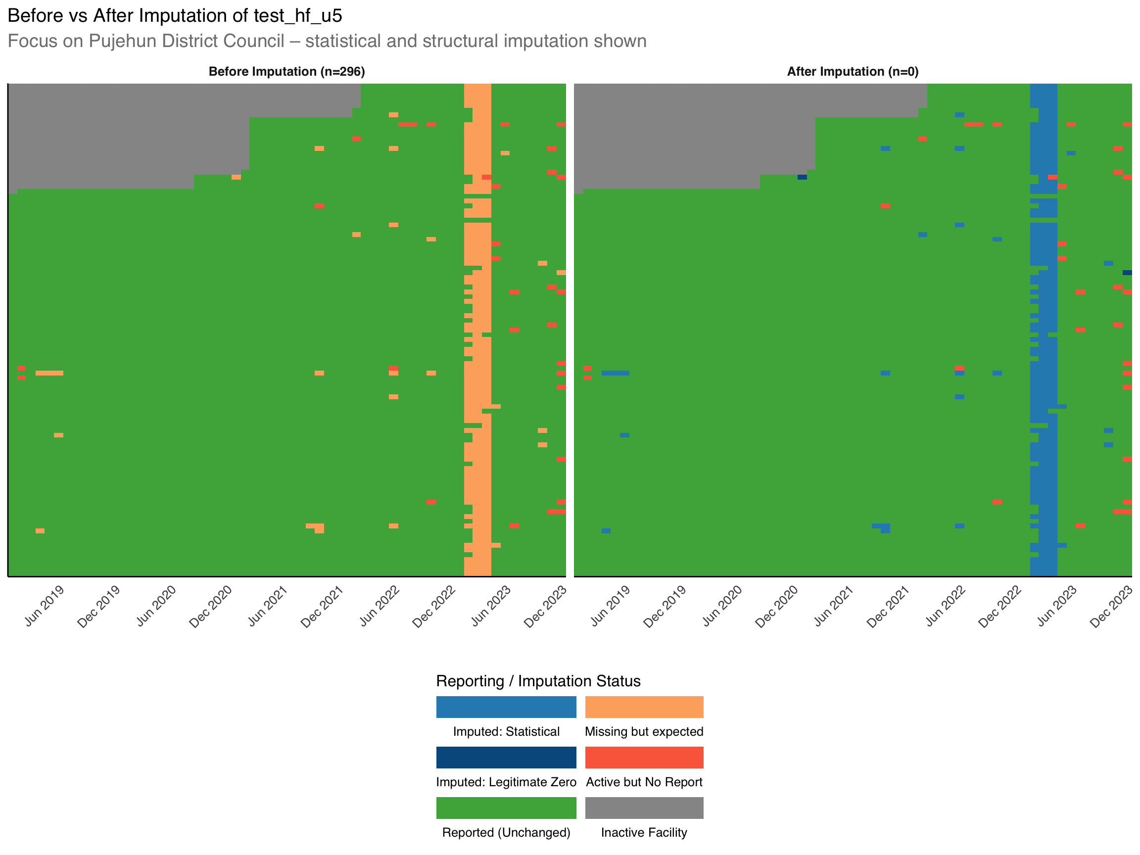
To adapt the code:
- Line 2: Replace
focus_districtwith your district of interest for visualization. - Lines 5-16: The statistical filters identify observations eligible for imputation analysis. Modify the grouping variable (
adm2) and detection patterns to match your data structure. - Lines 18-25: Update the facet labels and data selection to use your indicator names via the dynamic variable symbols.
The Moving Average imputation successfully filled 262 facility-month observations in Pujehun District and all other health facilities eligible for imputation.
Step 4.3: Comprehensive Imputation Summary
This section summarizes the final imputation status of each record in the dataset. Each record is labeled according to whether it was reported, imputed using a specific method, or remained missing.
Show the code
# classify imputation status across the dataset
# select key columns
final_data <- imputation_elig_stat |>
  dplyr::select(
    dplyr::any_of(names(df_routine)),
    !!var_final,
    !!var_imputed_name,
    imputation_status
  )

final_imputation_summary <- final_data |>
  dplyr::count(
    !!var_imputed_name,
    name = "n_records"
  ) |>
  dplyr::arrange(desc(n_records)) |>
  dplyr::mutate(
    percentage = round(n_records / sum(n_records) * 100, 1),
    n_records_formatted = scales::comma(n_records)
  )

knitr::kable(
  final_imputation_summary |>
    dplyr::select(!!var_imputed_name, n_records_formatted, percentage),
  caption = glue::glue(
    "Final Imputation Summary: Records by Method and Status for {var_to_impute}"
  ),
  col.names = c("Final Imputation Decision", "Count", "Percentage (%)")
)

n_total <- final_data |>
  nrow()

n_reported <- final_data |>
  dplyr::filter(!!var_imputed_name == "Reported (non-missing)") |>
  nrow()

n_imputed <- final_data |>
  dplyr::filter(
    stringr::str_detect(
      !!var_imputed_name,
      "Statistical imputation|Set to zero"
    )
  ) |>
  nrow()

imputation_rate <- round(n_imputed / n_total * 100, 1)
reporting_rate <- round(n_reported / n_total * 100, 1)

cli::cli_alert_info("Validation Results:")
cli::cli_alert_info("Total observations: {scales::comma(n_total)}")
cli::cli_alert_info(
  "Reported (non-missing): {scales::comma(n_reported)} ({reporting_rate}%)"
)
cli::cli_alert_info(
  "Successfully imputed: {scales::comma(n_imputed)} ({imputation_rate}%)"
)To adapt the code:
- Lines 4-8: Update the data selection to include your indicator’s final and decision variables using the dynamic variable symbols.
- Lines 10-16: The summary table uses the dynamic imputation decision variable to count and percentage outcomes by method. Modify the caption to reflect your specific indicator.
- Lines 18-30: Customize the validation statistics to match your reporting requirements. Adjust the pattern matching in
stringr::str_detect()to capture your specific imputation categories.
The imputation process for test_hf_u5 achieved comprehensive coverage with 73.1% of records already reported and requiring no imputation. Statistical imputation successfully filled 2.1% of missing observations, while legitimate zero imputation contributed minimally (0.0%). The remaining 24.8% were appropriately excluded from imputation due to inactive facilities (21.8%), facilities not reporting the indicator (2.7%), or indicators never being reported (0.2%).
ImportantValidate with SNT Team
Now that imputation is complete, validate the filled dataset with the SNT team. Cross-check summary tables, confirm suspicious patterns, and ensure key indicators behave as expected across districts and seasons. This step supports transparency and shared ownership of the results.
Step 5: Save Imputed Dataset
We save the imputed routine data for later use in analysis workflows.
# define save path
# save comprehensive imputed dataset as CSV
rio::export(
  final_data,
  here::here(
    data_path,
    "processed",
    "sle_test_comprehensive_imputed_routine_data_long.csv"
  )
)

# save comprehensive imputed dataset as RDS
rio::export(
  final_data,
  here::here(
    data_path,
    "processed",
    "sle_test_comprehensive_imputed_routine_data_long.rds"
  )
)

# save same dataset as parquet for python interop
arrow::write_parquet(
  final_data,
  here::here(
    data_path,
    "processed",
    "sle_test_comprehensive_imputed_routine_data_long.parquet"
  )
)

# save summary dataset
rio::export(
  final_imputation_summary,
  here::here(save_path, "sle_test_imputation_summary.csv")
)

# convert to wide format for analysis requiring wide structure
final_data_wide <- final_data |>
  dplyr::select(
    hf_uid,
    date,
    adm1,
    adm2,
    hf,
    test_original,
    test_final,
    fill_status_final
  ) |>
  tidyr::pivot_wider(
    id_cols = c(hf_uid, date, adm1, adm2, hf),
    names_from = "indicator", # assumes data includes indicator column
    values_from = c(test_original, test_final, fill_status_final),
    names_sep = "_"
  )

# save wide format dataset
rio::export(
  final_data_wide,
  here::here(
    data_path,
    "processed",
    "sle_test_comprehensive_imputed_routine_data_wide.csv"
  )
)

rio::export(
  final_data_wide,
  here::here(
    data_path,
    "processed",
    "sle_test_comprehensive_imputed_routine_data_wide.rds"
  )
)

# save wide format dataset as parquet for python interop
arrow::write_parquet(
  final_data_wide,
  here::here(
    data_path,
    "processed",
    "sle_test_comprehensive_imputed_routine_data_wide.parquet"
  )
)
To adapt the code:
- Lines 4-10, 14-20: Change file names to reflect your indicator, imputation method, and dataset specifics.
- Lines 30-40: Modify the wide format transformation to include the key variables you want to track for your indicator.
- Variable selection: Update the dataset to include your specific imputed variables and tracking columns.
The final imputed dataset combines all the systematic approaches demonstrated in this workflow. The saved dataset preserves both the original values and the imputed results, along with comprehensive tracking variables that document the imputation method applied to each observation. This transparency ensures that downstream analyses can appropriately account for imputed versus observed data and maintain analytical rigor.
The structured approach to missing data imputation demonstrated here provides a replicable framework for addressing surveillance data gaps while respecting epidemiological relationships and maintaining data quality standards.
Summary
This section provided a complete workflow for handling missing data in routine health facility reporting systems. We demonstrated how to systematically assess missingness patterns, distinguish between non-active facility status and true data gaps, and apply a comprehensive two-stage imputation approach.
The first stage applied structural imputation using epidemiological logic to infer missing values from downstream indicators (confirmed cases, treatments, admissions, deaths), identifying structural zeros and minimum-bound violations. The second stage employed statistical imputation methods, including constrained rolling means, to address remaining missing values while respecting epidemiological constraints and capturing temporal patterns.
Although this section focused on test_hf_u5 (aggregated malaria testing across age groups), the same approach applies to any routine indicator governed by similar reporting dependencies.
ImportantPost-Imputation Considerations
Three critical steps should be considered after completing the imputation process:
Recalculate aggregated and derived indicators: Imputed disaggregates (e.g.,
test_ov5) affect totals liketest, which must be updated to remain consistent. Similarly, derived columns likepresumedthat depend on other columns (e.g.,treatment) need recalculation.Consider recalculating reporting rates: Since imputed values directly affect whether indicators are considered reported, it may make sense to recalculate reporting rates to ensure consistency with the updated values.
Run post-imputation consistency checks: Even though constraint-based imputation helps safeguard against inconsistencies, implementing post-imputation validation checks is good practice to ensure imputation did not introduce any inconsistent values.
Full code
Find the full code script for imputing missing data in routine surveillance systems below.
Show full code
################################################################################
####################### ~ Imputation methods full code ~ #######################
################################################################################

### Step 1: Load Libraries and Read in Data ------------------------------------

#### Step 1.1: Install and load libraries --------------------------------------

# Install `pacman` if not already installed
if (!requireNamespace("pacman", quietly = TRUE)) {
  install.packages("pacman")
}

# Load required packages using pacman
pacman::p_load(
  dplyr,        # data manipulation
  ggplot2,      # plotting
  here,         # file path management
  lubridate,    # date handling
  tidyr,        # data reshaping
  cli,          # clean logging and CLI-style messages
  scales        # number formatting
)

#### Step 1.2: Load data -------------------------------------------------------

# set up data path
data_path <- here::here(
  "01_data", "1.2_epidemiology", "1.2a_routine_surveillance"
)

# read the processed surveillance data
df_routine <- readRDS(
  here::here(data_path, "processed", "clean_malaria_routine_data_final.rds")
) |>
  # filter to the past five years
  dplyr::filter(year >= 2019) |>
  dplyr::rename(maladm_hf_u5 = maladm_u5)

# preview the data
head(df_routine)

### Step 2: Determine HF Active vs. Non-Active Status --------------------------

#### Step 2.1: HF non-active status --------------------------------------------

# define key columns of interest
key_indicator_cols <- c(
  "test_hf_u5",
  "susp_hf_u5",
  "pres_hf_u5",
  "conf_hf_u5",
  "maltreat_hf_u5"
)

# generate full grid of all hf_uid and date combinations
full_grid <- tidyr::expand_grid(
  hf_uid = unique(df_routine$hf_uid),
  date = seq(min(df_routine$date), max(df_routine$date), by = "month")
)

# left join with your routine data
df_routine_balanced <- full_grid |>
  dplyr::left_join(df_routine, by = c("hf_uid", "date"))

# create reporting pattern analysis
routine_reporting_elig <- df_routine_balanced |>
  dplyr::mutate(
    # count how many indicators were reported (non-NA)
    indicators_reported = dplyr::across(dplyr::all_of(key_indicator_cols)) |>
      (\(x) rowSums(!is.na(x)))(),

    # mark rows where any indicator was reported
    reported_any = indicators_reported > 0
  ) |>
  dplyr::group_by(hf_uid) |>
  dplyr::mutate(
    # cumulative max to track if the facility has ever reported by that month
    has_ever_reported = cummax(reported_any),

    # date when the facility first reported any indicator
    first_reporting_date = if (any(reported_any)) {
      min(date[reported_any], na.rm = TRUE)
    } else {
      as.Date(NA)
    },
    #  classify each facility-month as 'active_reporting',
    # 'active_not_reporting', or 'inactive'
    activity_status = dplyr::case_when(
      reported_any ~ "Active Reporting",
      !reported_any & has_ever_reported ~ "Active Facility — Not Reporting",
      !reported_any & !has_ever_reported ~ "Inactive Facility"
    ),
    activity_status = factor(
      activity_status,
      level = c("Active Reporting", "Active Facility — Not Reporting", "Inactive Facility")
    )
  ) |>
  dplyr::ungroup()

# facility activeness plot
facility_activeness <-
  routine_reporting_elig |>
  dplyr::filter(!is.na(first_reporting_date)) |>
  ggplot2::ggplot(
    ggplot2::aes(
      x = date,
      y = forcats::fct_reorder(hf_uid, first_reporting_date),
      fill = activity_status
    )
  ) +
  ggplot2::geom_tile(
    width = 31,
    height = 1
  ) +
  ggplot2::scale_fill_manual(
    values = c(
      "Active Reporting" = "#1b9e77",
      "Active Facility — Not Reporting" = "#e7298a",
      "Inactive Facility" = "#d9d9d9"
    ),
    na.value = "grey90",
    name = "Reported any key indicator"
  ) +
  ggplot2::scale_x_date(
    expand = c(0, 0),
    date_labels = "%b %Y",
    date_breaks = "3 months"
  ) +
  ggplot2::labs(
    x = " ",
    y = NULL,
    title = glue::glue(
      "Monthly reporting activity by health facility ",
      "(n={format(dplyr::n_distinct(routine_reporting_elig$hf_uid),
      big.mark = \",\")})"
    )
  ) +
  ggplot2::theme_minimal(base_family = "sans") +
  ggplot2::guides(
    fill = ggplot2::guide_legend(
      title.position = "top",
      label.position = "bottom",
      keywidth = grid::unit(4.5, "lines")
    )
  ) +
  ggplot2::theme(
    axis.text.y = ggplot2::element_blank(),
    # axis.ticks.y = ggplot2::element_blank(),
    axis.line = ggplot2::element_line(color = "black", linewidth = 0.5),
    axis.text.x = ggplot2::element_text(angle = 45, hjust = 1),
    legend.position = "bottom",
    legend.direction = "horizontal",
    legend.box = "vertical"
  )

# display the plot
facility_activeness

# save plot
ggplot2::ggsave(
  plot = facility_activeness,
  here::here("03_output/3a_figures/sle_facility_activeness.png"),
  width = 12,
  height = 7,
  dpi = 300
)

#### Step 2.2: Apply clinical logic for structural imputation ------------------

# create never_reported flags for specific indicators using key_indicator_cols
never_reported_flags <- routine_reporting_elig |>
  dplyr::group_by(hf_uid) |>
  dplyr::summarise(
    never_reported_indicator = all(is.na(test_hf_u5)),
    .groups = "drop"
  )

# join back to main dataset and create imputation eligibility for test_hf_u5
imputation_elig <- routine_reporting_elig |>
  dplyr::left_join(never_reported_flags, by = "hf_uid") |>
  dplyr::mutate(
    # create imputation eligibility flag for test_hf_u5
    imputation_status = dplyr::case_when(
      activity_status == "Inactive Facility" ~ "Inactive Facility",
      never_reported_indicator == TRUE ~ "Indicator Never Reported",
      activity_status == "Active Facility — Not Reporting" ~ "Active Facility — Not Reporting",
      activity_status == "Active Reporting" &
        is.na(test_hf_u5) ~
        "Missing but Expected",
      activity_status == "Active Reporting" &
        !is.na(test_hf_u5) ~
        "Reported (non-missing)",
      TRUE ~ "Unknown"
    ),
    imputation_status = factor(
      imputation_status,
      levels = c(
        "Reported (non-missing)",
        "Missing but Expected",
        "Active Facility — Not Reporting",
        "Indicator Never Reported",
        "Inactive Facility",
        "Unknown"
      )
    )
  )

# get counts for legend labels
eligibility_counts <- imputation_elig |>
  dplyr::count(imputation_status) |>
  dplyr::mutate(
    label_with_n = paste0(
      imputation_status,
      " (n=",
      format(n, big.mark = ","),
      ")"
    )
  )

# create named vector for labels
legend_labels <- setNames(
  eligibility_counts$label_with_n,
  eligibility_counts$imputation_status
)

# create visualization showing imputation eligibility patterns
test_patterns <- imputation_elig |>
  dplyr::filter(!is.na(first_reporting_date)) |>
  dplyr::select(hf_uid, date, first_reporting_date, imputation_status)

# create imputation eligibility heatmap
imputation_eligibility_plot <- test_patterns |>
  ggplot2::ggplot(
    ggplot2::aes(
      x = date,
      y = forcats::fct_reorder(hf_uid, first_reporting_date),
      fill = imputation_status
    )
  ) +
  ggplot2::geom_tile(
    width = 31,
    height = 1
  ) +
  ggplot2::scale_fill_manual(
    values = c(
      "Reported (non-missing)" = "#1b9e77",
      "Missing but Expected" = "#ffdd57",
      "Active Facility — Not Reporting" = "#e66101",
      "Indicator Never Reported" = "#762a83",
      "Inactive Facility" = "#d9d9d9",
      "Unknown" = "#4575b4"
    ),
    labels = legend_labels,
    na.value = "white",
    name = "Imputation Status"
  ) +
  ggplot2::scale_x_date(
    expand = c(0, 0),
    date_labels = "%b %Y",
    date_breaks = "3 months"
  ) +
  ggplot2::labs(
    x = " ",
    y = NULL,
    title = "Imputation eligibility patterns for test_hf_u5 by health facility",
    subtitle = glue::glue(
      "Analysis of {format(dplyr::n_distinct(test_",
      "patterns$hf_uid), big.mark = ',')} facilities ",
      "showing data availability and imputation eligibility"
    )
  ) +
  ggplot2::theme_minimal(base_family = "sans", base_size = 12) +
  ggplot2::guides(
    fill = ggplot2::guide_legend(
      title.position = "top",
      label.position = "bottom",
      keywidth = grid::unit(3, "lines"),
      nrow = 2
    )
  ) +
  ggplot2::theme(
    axis.text.y = ggplot2::element_blank(),
    axis.line = ggplot2::element_line(color = "black", linewidth = 0.5),
    axis.text.x = ggplot2::element_text(angle = 45, hjust = 1),
    legend.position = "bottom",
    legend.direction = "horizontal",
    legend.box = "vertical",
    plot.subtitle = ggplot2::element_text(size = 14, color = "gray50")
  )

# display the plot
imputation_eligibility_plot

# save plot
ggplot2::ggsave(
  plot = imputation_eligibility_plot,
  here::here(
    "03_output/3a_figures/sle_test_imputation_eligibility_plot.png"
  ),
  width = 12,
  height = 7,
  dpi = 300
)

### Step 3: Resolve Missing Data -----------------------------------------------

#### Step 3.1: Structural imputation implementation (Stage 1) ------------------

# Get Upstream and Downstream Variables for Malaria Pathway Indicators
#
# Determines upstream and downstream variables for a given malaria indicator
# based on the clinical care pathway. Structural imputation is only allowed
# for indicators that follow predictable relationships in the pathway.
#
# Assumes variable names match standard: 'susp', 'test', 'conf',
# 'maltreat', 'maladm', 'maldth'.
#
# @param var_to_impute Character. Variable name to analyze (e.g., "conf").
#   Do not include suffix here; suffix is appended separately if provided.
# @param malaria_pathway Character vector. Ordered indicator sequence.
# @param facility_type Character or NULL. Facility type. Used to restrict
#   imputation for admissions ('maladm'), which only apply to inpatient-
#   capable facilities. Examples include: "hospital", "referral", "inpatient",
#   "health_facility" or "tertiary". All other facility types
#   (e.g., "health_post", "clinic") are treated as outpatient-only.
# @param suffix Character or NULL. Optional suffix to append to variable names
#   in output (e.g., "_hf" to return "test_hf", "conf_hf").
#
# @return A list with:
# \describe{
#   \item{var_to_impute}{Indicator with suffix applied.}
#   \item{upstream_vars}{Indicators that logically precede it.}
#   \item{downstream_vars}{Indicators that logically follow it.}
#   \item{use_structural}{Logical. TRUE if structural imputation is allowed.}
# }
#
# @details
# Indicator usage in imputation logic depends on facility type.
# Admissions ('maladm') are only included at inpatient-capable facilities.
## +------------+-----------------+--------------------+-----------------------+
## | Indicator  | Facility Type   | Upstream Used      | Downstream Used       |
## +------------+-----------------+--------------------+-----------------------+
#  | susp       | All             | —                  | test, conf, maladm*,  |
#  |            |                 |                    | maldth                |
#  | test       | All             | susp               | conf, maladm*, maldth |
#  | conf       | All             | susp, test         | maladm*, maldth       |
#  | maltreat   | All             | susp, test, conf   | maladm*, maldth       |
#  | maladm     | Inpatient only  | susp, test, conf   | maldth                |
#  | maladm     | Outpatient only | —                  | —                     |
#  | maldth     | All             | susp, test, conf,  |                       |
#  |            |                 | maladm*            | —                     |
## +------------+-----------------+--------------------+-----------------------+
# * Only used if facility is inpatient-capable
#
# @examples
# get_pathway_vars("test")
# get_pathway_vars("conf", suffix = "_hf")
# get_pathway_vars("maltreat")
# get_pathway_vars("maladm", facility_type = "hospital")
# get_pathway_vars("maladm", facility_type = "health_post")
#
# @export
get_pathway_vars <- function(
  var_to_impute,
  malaria_pathway = c("susp", "test", "conf", "maltreat", "maladm", "maldth"),
  facility_type = NULL,
  suffix = NULL
) {
  append_suffix <- function(x) {
    if (length(x) == 0) {
      character()
    } else if (is.null(suffix)) {
      x
    } else {
      paste0(x, suffix)
    }
  }

  inpatient_types <- c("hospital", "referral", "inpatient", "tertiary")

  if (var_to_impute == "maladm") {
    is_inpatient <- !is.null(facility_type) &&
      tolower(facility_type) %in% tolower(inpatient_types)

    if (!is_inpatient) {
      cli::cli_h1("Malaria Pathway Summary")
      cli::cli_alert_info(
        "Imputing for {.field {append_suffix(var_to_impute)}}"
      )
      cli::cli_alert_danger(
        "Admissions not applicable at outpatient facilities (e.g., health post)."
      )
      cli::cli_alert_warning("Structural imputation excluded")
      cli::cli_alert_success("Upstream: None")
      cli::cli_alert_success("Downstream: None")

      return(list(
        var_to_impute = append_suffix(var_to_impute),
        upstream_vars = character(),
        downstream_vars = character(),
        use_structural = FALSE
      ))
    }
  }

  is_inpatient <- !is.null(facility_type) &&
    tolower(facility_type) %in% tolower(inpatient_types)

  non_linear <- character()
  if (var_to_impute != "maltreat") {
    non_linear <- c(non_linear, "maltreat")
  }
  if (!is_inpatient) {
    non_linear <- c(non_linear, "maladm")
  }

  linear_path <- malaria_pathway[!malaria_pathway %in% non_linear]
  pos <- match(var_to_impute, linear_path)

  upstream_vars <- if (is.na(pos) || pos <= 1) {
    character()
  } else {
    linear_path[1:(pos - 1)]
  }

  downstream_vars <- if (is.na(pos) || pos >= length(linear_path)) {
    character()
  } else {
    linear_path[(pos + 1):length(linear_path)]
  }

  upstream_str <- if (length(upstream_vars) == 0) {
    "None"
  } else {
    paste(append_suffix(upstream_vars), collapse = ", ")
  }
  downstream_str <- if (length(downstream_vars) == 0) {
    "None"
  } else {
    paste(append_suffix(downstream_vars), collapse = ", ")
  }

  cli::cli_h1("Malaria Pathway Summary")
  cli::cli_alert_info("Imputing for {.field {append_suffix(var_to_impute)}}")
  cli::cli_alert_success("Upstream: {.field {upstream_str}}")
  cli::cli_alert_success("Downstream: {.field {downstream_str}}")

  if (
    var_to_impute != "maladm" &&
      "maladm" %in% malaria_pathway &&
      !is_inpatient
  ) {
    cli::cli_alert_info(
      paste0(
        "Note: {.val ",
        append_suffix("maladm"),
        "} excluded from dependency logic due to outpatient facility."
      )
    )
  }

  if (
    var_to_impute != "maltreat" &&
      "maltreat" %in% malaria_pathway
  ) {
    cli::cli_alert_info(
      paste0(
        "Note: {.val ",
        append_suffix("maltreat"),
        "} excluded from dependency logic due to presumptive treatment."
      )
    )
  }

  cli::cat_line()

  return(list(
    var_to_impute = append_suffix(var_to_impute),
    upstream_vars = append_suffix(upstream_vars),
    downstream_vars = append_suffix(downstream_vars),
    use_structural = TRUE
  ))
}

# get upstream and downstream indicators
ud_test_hf <- get_pathway_vars(
  var_to_impute = "test",
  malaria_pathway = c("susp", "test", "conf", "maltreat", "maladm", "maldth"),
  suffix = "_hf_u5",
  facility_type = "hospital"

# extract dynamic components from the pathway definition
upstream_vars <- ud_test_hf$upstream_vars
downstream_vars <- ud_test_hf$downstream_vars
use_structural <- ud_test_hf$use_structural
var_to_impute <- rlang::sym(ud_test_hf$var_to_impute)

imputation_elig_str <- imputation_elig |>
  dplyr::mutate(
    # binary column determining whether var_to_impute requires imputation
    to_impute = coalesce(imputation_status == "Missing but Expected", FALSE),
    # check the existence of positive downstream
    has_positive_upstream = if (length(upstream_vars) == 0L) {
      FALSE
    } else {
      rowSums(
        dplyr::across(
          dplyr::any_of(upstream_vars),
          ~ (!is.na(.x) & .x > 0) + 0L
        ),
        na.rm = TRUE
      ) >
        0
    },
    # check the existence of positive upstream
    has_positive_downstream = if (length(downstream_vars) == 0L) {
      FALSE
    } else {
      rowSums(
        dplyr::across(
          dplyr::any_of(downstream_vars),
          ~ (!is.na(.x) & .x > 0) + 0L
        ),
        na.rm = TRUE
      ) >
        0
    },
  ) |>
  # classify structural pattern based on logic
  dplyr::mutate(
    structural_classification = dplyr::case_when(
      !is.na({{ var_to_impute }}) ~ "Value observed",
      to_impute &
        is.na({{ var_to_impute }}) &
        !has_positive_upstream &
        !has_positive_downstream ~
        "No pathway evidence reported",
      to_impute & is.na({{ var_to_impute }}) & has_positive_downstream ~
        "Positive downstream indicators reported",
      to_impute &
        is.na({{ var_to_impute }}) &
        has_positive_upstream &
        !has_positive_downstream ~
        "Positive upstream reported, no downstream evidence",
      !to_impute ~ "Not eligible for imputation",
      TRUE ~ "Pattern unclear"
    )
  ) |>
  # compute rowwise max from downstream indicators
  dplyr::mutate(
    max_downstream = if (length(downstream_vars) == 0L) {
      NA_real_
    } else {
      raw <- do.call(
        pmax,
        c(
          as.list(dplyr::select(
            cur_data_all(),
            dplyr::any_of(downstream_vars)
          )),
          na.rm = TRUE
        )
      )
      raw[is.infinite(raw) & raw < 0] <- NA_real_
      raw
    }
  ) |>
  dplyr::ungroup() |>

  # apply minimum constraint where relevant
  dplyr::mutate(
    minimum_constraint = dplyr::case_when(
      has_positive_downstream & is.na({{ var_to_impute }}) ~ max_downstream,
      TRUE ~ NA_real_
    )
  ) |>
  # pre-compute matching downstream variable for cleaner logic
  dplyr::mutate(
    matching_downstream = {
      matches <- downstream_vars[downstream_vars == max_downstream]
      if (length(matches) == 1) {
        matches
      } else {
        "Statistical imputation (constrained)"
      }
    },
    imputation_source = dplyr::case_when(
      !is.na({{ var_to_impute }}) ~ "Original value",
      structural_classification == "No pathway evidence reported" ~
        "Set to zero (imputation)",
      structural_classification == "Positive downstream indicators reported" ~
        matching_downstream,
      structural_classification == "Not eligible for imputation" ~
        "None - no imputation",
      TRUE ~ "Statistical imputation"
    )
  ) |>
  dplyr::select(-matching_downstream) |>
  # flag unclear or uncertain cases
  dplyr::mutate(
    needs_review = structural_classification %in%
      c(
        "Positive downstream indicators reported",
        "Positive upstream reported, no downstream evidence",
        "Pattern unclear"
      )
  )

# impute legitimate zero rows to 0
imputation_elig_str <- imputation_elig_str |>
  dplyr::mutate(
    "{var_to_impute}_structural" := dplyr::if_else(
      imputation_source == "Set to zero (imputation)",
      0,
      {{ var_to_impute }}
    )
  )

# display classification summary
imputation_elig_str |>
  dplyr::filter(structural_classification != "Not eligible for imputation") |>
  dplyr::count(structural_classification, imputation_source, sort = TRUE) |>
  dplyr::mutate(Count = scales::comma(n)) |>
  dplyr::select(
    `Structural Classification` = structural_classification,
    `Imputation Source` = imputation_source,
    Count
  ) |>
  knitr::kable(
    caption = glue::glue(
      "Summary of Structural Classifications and Sources Used ",
      "in Imputing Missing `{var_to_impute}` Values"
    )
  )

#### Step 3.2: Implement constrained moving average imputation (Stage 2) -------

# create variable names for injection and symbols for cleaner injection
var_roll_primary <- paste0(var_to_impute, "_roll_primary") |> rlang::sym()
var_fallback <- paste0(var_to_impute, "_fallback") |> rlang::sym()
var_original <- paste0(var_to_impute, "_original") |> rlang::sym()
var_imp_stat <- paste0(var_to_impute, "_imp_stat") |> rlang::sym()
var_final <- paste0(var_to_impute, "_final") |> rlang::sym()
var_structural <- paste0(var_to_impute, "_structural") |> rlang::sym()
var_to_impute_sym <- var_to_impute |> rlang::sym()
var_imputed_name <- paste0(var_to_impute, "_final_decision") |> rlang::sym()

# constrained moving average imputation
imputation_elig_stat <- imputation_elig_str |>
  dplyr::arrange(hf_uid, date) |>
  dplyr::mutate(
    !!var_roll_primary := zoo::rollmean(
      !!var_structural,
      k = 3,
      fill = NA,
      align = "right"
    ) |>
      round()
  ) |>
  dplyr::ungroup() |>
  # compute fallback (adm3-level) rolling means
  dplyr::group_by(adm2) |>
  dplyr::mutate(
    !!var_fallback := zoo::rollmean(
      !!var_structural,
      k = 3,
      fill = NA,
      align = "right"
    ) |>
      round()
  ) |>
  dplyr::ungroup() |>
  # impute using the available rolling mean + constraint
  dplyr::mutate(
    !!var_original := test,
    !!var_imp_stat := dplyr::case_when(
      !is.na(!!var_roll_primary) ~
        pmax(!!var_roll_primary, minimum_constraint, na.rm = TRUE),
      !is.na(!!var_fallback) ~
        pmax(!!var_fallback, minimum_constraint, na.rm = TRUE),
      TRUE ~ minimum_constraint
    ),
    !!var_final := dplyr::case_when(
      # get non missing
      !is.na(!!var_to_impute_sym) ~ !!var_to_impute_sym,
      # first impute with structural zeros
      is.na(!!var_to_impute_sym) & !is.na(!!var_structural) ~ !!var_structural,
      # then impute with rolling mean
      is.na(!!var_to_impute_sym) &
        is.na(!!var_structural) &
        !is.na(!!var_roll_primary) ~
        !!var_roll_primary,
      # fallback option
      is.na(!!var_to_impute_sym) &
        is.na(!!var_structural) &
        is.na(!!var_roll_primary) &
        !is.na(!!var_fallback) ~
        !!var_fallback,
      # final fallback
      TRUE ~ minimum_constraint
    )
  ) |>
  # declare final imputation method used
  dplyr::mutate(
    # create comprehensive imputation flag using generic name
    !!var_imputed_name := dplyr::case_when(
      imputation_status == "Active Facility — Not Reporting" ~
        "No imputation (not reporting indicator)",
      imputation_status == "Indicator Never Reported" ~
        "No imputation (indicator never reported)",
      imputation_status == "Inactive Facility" ~
        "No imputation (inactive facility)",
      imputation_status == "Missing but Expected" &
        imputation_source == "Statistical imputation" ~
        "Statistical imputation",
      imputation_status == "Missing but Expected" &
        imputation_source == "Set to zero (imputation)" ~
        "Set to zero (imputation)",
      imputation_status == "Missing but Expected" &
        imputation_source == "Statistical imputation (constrained)" ~
        "Statistical imputation (constrained)",
      is.na(!!var_to_impute_sym) ~ "Not imputed",
      TRUE ~ imputation_status
    ),
    !!var_imputed_name := factor(
      !!rlang::sym(var_imputed_name),
      levels = c(
        "Reported (non-missing)",
        "No imputation (inactive facility)",
        "No imputation (not reporting indicator)",
        "No imputation (indicator never reported)",
        "Statistical imputation",
        "Statistical imputation (constrained)",
        "Set to zero (imputation)",
        "Not imputed"
      )
    )
  )

# check final out
knitr::kable(
  imputation_elig_stat |>
    dplyr::count(!!var_imputed_name) |>
    dplyr::mutate(n = scales::comma(n)) |>
    dplyr::arrange(desc(n)) |>
    dplyr::rename(
      `Final Imputation Decision` = !!var_imputed_name,
      `Number of Observations` = n
    ),
  caption = glue::glue(
    "Summary of Final Imputation Decisions Made for `{var_to_impute}` Values"
  )
)

# establish district to focus on
focus_district <- "PUJEHUN"

# get total imputations to be done in given district
n_total <- imputation_elig_stat |>
  dplyr::filter(
    adm2 == focus_district,
    stringr::str_detect(!!var_imputed_name, "Statistical imputation"),
    !is.na(first_reporting_date),
    is.na(!!var_to_impute_sym)
  ) |>
  dplyr::distinct(hf_uid, date) |>
  nrow()

# get total imputations done in given district
n_imputed <- imputation_elig_stat |>
  dplyr::filter(
    adm2 == focus_district,
    stringr::str_detect(!!var_imputed_name, "Statistical imputation"),
    !is.na(first_reporting_date)
  ) |>
  dplyr::distinct(hf_uid, date) |>
  nrow()

# define custom labels for facet display
facet_labels <- c(
  "Before" = paste0(
    "Before Imputation (n=",
    format(n_total, big.mark = ","),
    ")"
  ),
  "After" = paste0(
    "After Imputation (n=",
    format(n_total - n_imputed, big.mark = ","),
    ")"
  )
)

# create comparison data
imputation_comparison <- imputation_elig_stat |>
  dplyr::filter(
    !is.na(first_reporting_date),
    adm2 == focus_district
  ) |>
  dplyr::select(
    hf_uid,
    date,
    first_reporting_date,
    !!var_original,
    !!var_final,
    !!var_imputed_name,
    imputation_status,
    hf
  ) |>
  tidyr::pivot_longer(
    cols = c(!!var_original, !!var_final),
    names_to = "name",
    values_to = "indicator_value"
  ) |>
  dplyr::mutate(
    imputation_stage = dplyr::case_when(
      name == paste0(var_to_impute, "_original") ~ "Before",
      name == paste0(var_to_impute, "_final") ~ "After"
    ),
    imputation_stage = factor(
      imputation_stage,
      levels = c("Before", "After")
    ),
    fill_status = dplyr::case_when(
      !is.na(indicator_value) &
        imputation_status == "Reported (non-missing)" ~
        "Reported (Unchanged)",
      imputation_stage == "After" &
        !!var_imputed_name %in%
          c(
            "Statistical imputation",
            "Statistical imputation (constrained)"
          ) ~
        "Imputed: Statistical",
      imputation_stage == "Before" &
        !!var_imputed_name %in%
          c(
            "Set to zero (imputation)",
            "Statistical imputation",
            "Statistical imputation (constrained)"
          ) ~
        "Missing but expected",
      imputation_stage == "After" &
        !!var_imputed_name == "Set to zero (imputation)" ~
        "Imputed: Legitimate Zero",
      !!var_imputed_name == "No imputation (inactive facility)" ~
        "Inactive Facility",
      !!var_imputed_name == "No imputation (not reporting indicator)" ~
        "Active but No Report",
      !!var_imputed_name == "No imputation (indicator never reported)" ~
        "Indicator Never Reported",
      imputation_stage == "Before" & is.na(indicator_value) ~
        "Missing but expected",
      TRUE ~ "Other / Unclassified"
    ),
    ,

    fill_status = factor(
      fill_status,
      levels = c(
        "Imputed: Statistical",
        "Imputed: Legitimate Zero",
        "Reported (Unchanged)",
        "Missing but expected",
        "Active but No Report",
        "Indicator Never Reported",
        "Inactive Facility",
        "Other / Unclassified"
      )
    )
  )

# create comparison plot
before_after_plot <- ggplot2::ggplot(
  imputation_comparison,
  ggplot2::aes(
    x = date,
    y = forcats::fct_reorder(hf, first_reporting_date),
    na.rm = TRUE,
    fill = fill_status
  )
) +
  ggplot2::geom_tile(width = 31, height = 1) +
  ggplot2::facet_wrap(
    ~imputation_stage,
    ncol = 2,
    labeller = ggplot2::as_labeller(facet_labels)
  ) +
  ggplot2::scale_fill_manual(
    values = c(
      "Imputed: Statistical" = "#2b8cbe",
      "Imputed: Legitimate Zero" = "#045a8d",
      "Reported (Unchanged)" = "#4daf4a",
      "Missing but expected" = "#fdae6b",
      "Active but No Report" = "#fb6a4a",
      "Indicator Never Reported" = "#d62728",
      "Inactive Facility" = "#969696",
      "Other / Unclassified" = "#6a3d9a"
    ),
    name = "Reporting / Imputation Status"
  ) +
  ggplot2::scale_x_date(
    expand = c(0, 0),
    date_labels = "%b %Y",
    date_breaks = "6 months"
  ) +
  ggplot2::labs(
    x = "",
    y = NULL,
    title = glue::glue("Before vs After Imputation of {var_to_impute}"),
    subtitle = paste0(
      "Focus on ",
      focus_district,
      " – statistical and structural imputation shown"
    )
  ) +
  ggplot2::theme_minimal(base_family = "sans", base_size = 12) +
  ggplot2::guides(
    fill = ggplot2::guide_legend(
      title.position = "top",
      label.position = "bottom",
      keywidth = grid::unit(3, "lines"),
      nrow = 3
    )
  ) +
  ggplot2::theme(
    axis.text.y = ggplot2::element_blank(),
    axis.line = ggplot2::element_line(
      color = "black",
      linewidth = 0.5
    ),
    axis.text.x = ggplot2::element_text(angle = 45, hjust = 1),
    legend.position = "bottom",
    legend.direction = "horizontal",
    legend.box = "vertical",
    strip.text = ggplot2::element_text(face = "bold"),
    plot.subtitle = ggplot2::element_text(size = 14, color = "gray50")
  )

# display the plot
before_after_plot

# save plot
ggplot2::ggsave(
  plot = before_after_plot,
  here::here("03_output/3a_figures/sle_test_before_after_plot.png"),
  width = 12,
  height = 7,
  dpi = 300
)

#### Step 3.3: Comprehensive imputation summary --------------------------------

# classify imputation status across the dataset
# select key columns
final_data <- imputation_elig_stat |>
  dplyr::select(
    dplyr::any_of(names(df_routine)),
    !!var_final,
    !!var_imputed_name,
    imputation_status
  )

final_imputation_summary <- final_data |>
  dplyr::count(
    !!var_imputed_name,
    name = "n_records"
  ) |>
  dplyr::arrange(desc(n_records)) |>
  dplyr::mutate(
    percentage = round(n_records / sum(n_records) * 100, 1),
    n_records_formatted = scales::comma(n_records)
  )

knitr::kable(
  final_imputation_summary |>
    dplyr::select(!!var_imputed_name, n_records_formatted, percentage),
  caption = glue::glue(
    "Final Imputation Summary: Records by Method and Status for {var_to_impute}"
  ),
  col.names = c("Final Imputation Decision", "Count", "Percentage (%)")
)

n_total <- final_data |>
  nrow()

n_reported <- final_data |>
  dplyr::filter(!!var_imputed_name == "Reported (non-missing)") |>
  nrow()

n_imputed <- final_data |>
  dplyr::filter(
    stringr::str_detect(
      !!var_imputed_name,
      "Statistical imputation|Set to zero"
    )
  ) |>
  nrow()

imputation_rate <- round(n_imputed / n_total * 100, 1)
reporting_rate <- round(n_reported / n_total * 100, 1)

cli::cli_alert_info("Validation Results:")
cli::cli_alert_info("Total observations: {scales::comma(n_total)}")
cli::cli_alert_info(
  "Reported (non-missing): {scales::comma(n_reported)} ({reporting_rate}%)"
)
cli::cli_alert_info(
  "Successfully imputed: {scales::comma(n_imputed)} ({imputation_rate}%)"
)

### Step 4: Save Imputed Dataset -----------------------------------------------

# define save path
# save comprehensive imputed dataset as CSV
rio::export(
  final_data,
  here::here(
    data_path,
    "processed",
    "sle_test_comprehensive_imputed_routine_data_long.csv"
  )
)

# save comprehensive imputed dataset as RDS
rio::export(
  final_data,
  here::here(
    data_path,
    "processed",
    "sle_test_comprehensive_imputed_routine_data_long.rds"
  )
)

# save summary dataset
rio::export(
  final_imputation_summary,
  here::here(data_path, "processed", "sle_test_imputation_summary.csv")
)

# convert to wide format for analysis requiring wide structure
final_data_wide <- final_data |>
  dplyr::select(
    hf_uid,
    date,
    adm1,
    adm2,
    hf,
    test_original,
    test_final,
    fill_status_final
  ) |>
  tidyr::pivot_wider(
    id_cols = c(hf_uid, date, adm1, adm2, hf),
    names_from = "indicator", # assumes data includes indicator column
    values_from = c(test_original, test_final, fill_status_final),
    names_sep = "_"
  )

# save wide format dataset
rio::export(
  final_data_wide,
  here::here(
    data_path,
    "processed",
    "sle_test_comprehensive_imputed_routine_data_wide.csv"
  )
)

rio::export(
  final_data_wide,
  here::here(
    data_path,
    "processed",
    "sle_test_comprehensive_imputed_routine_data_wide.rds"
  )
)