################################### Option 1 ###################################
#===============================================================================
# Step 1.1: Set-Up and Download DHS data
#===============================================================================
# install or load required packages
pacman::p_load(
  here,       # For handling relative file paths
  haven,      # For reading DHS .dta files and labelled data
  dplyr,      # For data wrangling
  stringr,    # For filtering U5MR rows using regex
  tibble,     # For rownames_to_column
  ggplot2,    # For visualizing U5MR maps
  sf,         # For working with shapefiles
  rio,        # For saving outputs in .csv and .rds formats
  DHS.rates   # For calculating under-five mortality rates
)

#' Check DHS Indicator List from API
#'
#' @param countryIds DHS country code(s), e.g., "EG"
#' @param indicatorIds Specific indicator ID(s)
#' @param surveyIds Survey ID(s)
#' @param surveyYear Exact year
#' @param surveyYearStart Start of year range
#' @param surveyYearEnd End of year range
#' @param surveyType DHS survey type (e.g., "DHS", "MIS")
#' @param surveyCharacteristicIds Filter by survey characteristic ID
#' @param tagIds Filter by tag ID
#' @param returnFields Fields to return (default: IndicatorId, Label, Definition)
#' @param perPage Max results per page (default = 500)
#' @param page Specific page to return (default = 1)
#' @param f Format (default = "json")
#'
#' @return A data.frame of indicators
#' @export
check_dhs_indicators <- function(
  countryIds = NULL,
  indicatorIds = NULL,
  surveyIds = NULL,
  surveyYear = NULL,
  surveyYearStart = NULL,
  surveyYearEnd = NULL,
  surveyType = NULL,
  surveyCharacteristicIds = NULL,
  tagIds = NULL,
  returnFields = c("IndicatorId", "Label", "Definition", "MeasurementType"),
  perPage = NULL,
  page = NULL,
  f = "json"
) {
  # Base URL
  base_url <- "https://api.dhsprogram.com/rest/dhs/indicators?"

  # Build query string
  params <- list(
    countryIds = countryIds,
    indicatorIds = indicatorIds,
    surveyIds = surveyIds,
    surveyYear = surveyYear,
    surveyYearStart = surveyYearStart,
    surveyYearEnd = surveyYearEnd,
    surveyType = surveyType,
    surveyCharacteristicIds = surveyCharacteristicIds,
    tagIds = tagIds,
    returnFields = paste(returnFields, collapse = ","),
    perPage = perPage,
    page = page,
    f = f
  )

  # Drop NULLs and encode
  query <- paste(
    purrr::compact(params) |>
      purrr::imap_chr(
        ~ paste0(.y, "=", URLencode(as.character(.x), reserved = TRUE))
      ),
    collapse = "&"
  )

  # Full URL
  full_url <- paste0(base_url, query)

  # Fetch with progress bar
  response <- httr::GET(full_url, httr::progress())
  jsonlite::fromJSON(httr::content(
    response,
    as = "text",
    encoding = "UTF-8"
  ))$Data
}

#' Query DHS API Directly via URL Parameters
#'
#' Builds and queries DHS API for indicator data using URL-based access
#' instead of rdhs package.
#'
#' @param countryIds Comma-separated DHS country code(s), e.g., "SL"
#' @param indicatorIds Comma-separated DHS indicator ID(s), e.g., "CM_ECMR_C_U5M"
#' @param surveyIds Optional comma-separated survey ID(s), e.g., "SL2016DHS"
#' @param surveyYear Optional exact survey year, e.g., "2016"
#' @param surveyYearStart Optional survey year range start
#' @param surveyYearEnd Optional survey year range end
#' @param breakdown One of: "national", "subnational", "background", "all"
#' @param f Format to return (default is "json")
#'
#' @return A data.frame containing the `Data` portion of the API response.
#' @export
download_dhs_indicators <- function(
  countryIds,
  indicatorIds,
  surveyIds = NULL,
  surveyYear = NULL,
  surveyYearStart = NULL,
  surveyYearEnd = NULL,
  breakdown = "subnational",
  f = "json"
) {
  # Base URL
  base_url <- "https://api.dhsprogram.com/rest/dhs/data?"

  # Assemble query string
  query <- paste0(
    "breakdown=",
    breakdown,
    "&indicatorIds=",
    indicatorIds,
    "&countryIds=",
    countryIds,
    if (!is.null(surveyIds)) paste0("&surveyIds=", surveyIds),
    if (!is.null(surveyYear)) paste0("&surveyYear=", surveyYear),
    if (!is.null(surveyYearStart)) paste0("&surveyYearStart=", surveyYearStart),
    if (!is.null(surveyYearEnd)) paste0("&surveyYearEnd=", surveyYearEnd),
    "&lang=en&f=",
    f
  )

  full_url <- paste0(base_url, query)

  cli::cli_alert_info("Downloading DHS data...")

  response <- httr::GET(full_url, httr::progress())

  if (httr::http_error(response)) {
    stop("API request failed: ", httr::status_code(response))
  }

  content_raw <- httr::content(response, as = "text", encoding = "UTF-8")
  data <- jsonlite::fromJSON(content_raw)$Data

  cli::cli_alert_success("Download complete: {nrow(data)} records retrieved.")
  return(data)
}
#===============================================================================
# Step 1.2: Download the Relevant Indicators
#===============================================================================
# get mean Under-five mortality rate at subnational level
u5mr_mean_dhs_ind <- download_dhs_indicators(
  countryIds = "SL",
  surveyYear = 2019,
  indicatorIds = "CM_ECMR_C_U5M",
  breakdown = "subnational"
) |>
  dplyr::mutate(
    dhs_indicator_id = "CM_ECMR_C_U5M",
    indicator = "Under-five mortality rate"
  ) |>
  dplyr::select(
    dhs_indicator_id,
    indicator,
    adm2_code = RegionId,
    mean_u5mr = Value
  )

# get lower interval Under-five mortality rate at subnational level
u5mr_low_dhs_ind <- download_dhs_indicators(
  countryIds = "SL",
  surveyYear = 2019,
  indicatorIds = "CM_ECMR_C_U5L",
  breakdown = "subnational"
) |>
  dplyr::mutate(
    dhs_indicator_id = "CM_ECMR_C_U5L",
    indicator = "Under-five mortality rate"
  ) |>
  dplyr::select(
    adm2_code = RegionId,
    low_u5mr = Value
  )

# get upper interval Under-five mortality rate at subnational level
u5mr_upp_dhs_ind <- download_dhs_indicators(
  countryIds = "SL",
  surveyYear = 2019,
  indicatorIds = "CM_ECMR_C_U5U",
  breakdown = "subnational"
) |>
  dplyr::mutate(
    dhs_indicator_id = "CM_ECMR_C_U5U",
    indicator = "Under-five mortality rate"
  ) |>
  dplyr::select(
    adm2_code = RegionId,
    upp_u5mr = Value
  )
#===============================================================================
# Step 1.3: Join Indicators with Shapefile
#===============================================================================
# get the DHS adm2 shapefile
sle_dhs_shp2 <- sf::read_sf(
  here::here(
    "01_foundational/1a_administrative_boundaries",
    "1ai_adm2",
    "sdr_subnational_boundaries_adm2.shp"
  )
) |>
  dplyr::select(
    adm1 = OTHREGNA,
    adm2 = DHSREGEN,
    adm2_code = REG_ID
  ) |>
  # make adm1 and adm2 to upper case
  dplyr::mutate(
    adm1 = toupper(adm1),
    adm2 = toupper(adm2)
  )

# join the mean, conficte intevals u5mr estimates
dhs_api_indi <- u5mr_mean_dhs_ind |>
  dplyr::left_join(u5mr_low_dhs_ind, by = "adm2_code") |>
  dplyr::left_join(u5mr_upp_dhs_ind, by = "adm2_code") |>
  # join adm2 dhs shapefile to data only keeping adm2 indicators
  dplyr::inner_join(sle_dhs_shp2, by = "adm2_code") |>
  # select only relevant columns
  dplyr::select(
    dhs_indicator_id,
    indicator,
    adm1,
    adm2,
    mean_u5mr,
    low_u5mr,
    upp_u5mr,
    geometry
  ) |>
  sf::st_as_sf()

# check indicators
sf::st_drop_geometry(dhs_api_indi)
#===============================================================================
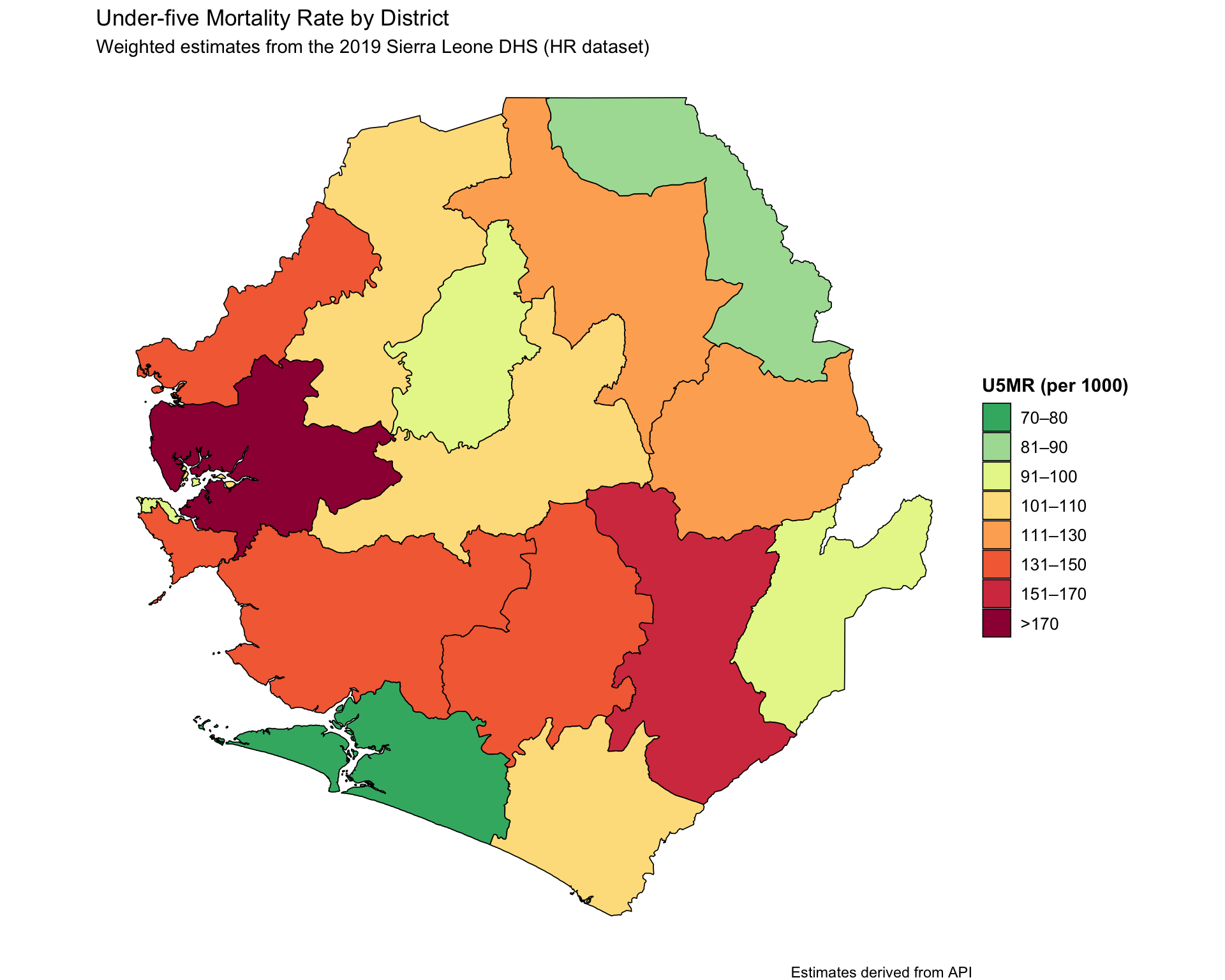
# Step 1.4: Visualize Subnational Indicator Data
#===============================================================================
u5mr_final_api <- dhs_api_indi |>
dplyr::mutate(
prop_cat = cut(
mean_u5mr,
breaks = c(0, 80, 90, 100, 110, 130, 150, 170, Inf),
labels = c(
"70–80",
"81–90",
"91–100",
"101–110",
"111–130",
"131–150",
"151–170",
">170"
),
include.lowest = TRUE,
right = FALSE
)
)
# visualise the U5MR results
map_u5mr <- u5mr_final_api |>
ggplot2::ggplot() +
ggplot2::geom_sf(
ggplot2::aes(fill = prop_cat, geometry = geometry),
color = "black",
size = 0.3,
show.legend = TRUE
) +
ggplot2::scale_fill_manual(
name = "U5MR (per 1000)",
values = c(
">170" = "#9E0142",
"151–170" = "#D53E4F",
"131–150" = "#F46D43",
"111–130" = "#FDAE61",
"101–110" = "#FEE08B",
"91–100" = "#E6F598",
"81–90" = "#ABDDA4",
"70–80" = "#3CB371"
),
drop = FALSE
) +
ggplot2::labs(
title = "Under-five Mortality Rate by District",
subtitle = "Weighted estimates from the 2019 Sierra Leone DHS (HR dataset)",
caption = "Estimates derived from API"
) +
ggplot2::theme_void() +
ggplot2::theme(
legend.title = ggplot2::element_text(face = "bold"),
legend.text = ggplot2::element_text(size = 10)
)
################################### Option 2 ###################################
#===============================================================================
# Step 2.1: Load the Relevant DHS Data
#===============================================================================
# import the KR (childrens) data
sle_dhs_kr <- readRDS(
here::here("1.6_health_systems/1.6a_dhs/raw/SLKR7AFL.rds")
) |>
# make location col
dplyr::mutate(
adm1 = haven::as_factor(v024) |>
toupper(),
adm2 = haven::as_factor(sdist) |>
toupper(),
location = paste0(adm1, ", ", adm2)
)
# get the DHS adm2 shapefile
sle_dhs_shp2 <- sf::read_sf(
here::here(
"01_foundational/1a_administrative_boundaries",
"1ai_adm2",
"sdr_subnational_boundaries_adm2.shp"
)
) |>
dplyr::select(
adm1 = OTHREGNA,
adm2 = DHSREGEN,
adm2_code = REG_ID
) |>
# make adm1 and adm2 to upper case
dplyr::mutate(
adm1 = toupper(adm1),
adm2 = toupper(adm2)
)
#===============================================================================
# Step 2,2: Calculate U5MR at District Level
#===============================================================================
# calculate five-year under-five mortality rates
mort_sl <- sle_dhs_kr |>
DHS.rates::chmort(
JK = "Yes", # For getting confidence intervals
Strata = "v022", # Strata variable for complex survey design
Cluster = "v021", # Cluster (PSU) identifier
Weight = "v005", # Sampling weight
Date_of_interview = "v008", # Date of interview (CMC format)
Date_of_birth = "b3", # Child’s date of birth (CMC format)
Class = "location" # Grouping variable (e.g., region, district)
)
mort_sl
#===============================================================================
# Step 2.3: Prepare Subnational U5MR for plotting
#===============================================================================
mort_sl2 <- mort_sl |>
tibble::rownames_to_column(var = "type") |> # convert rownames to a column
dplyr::filter(stringr::str_detect(type, "U5MR")) |> # keep only U5MR rows
dplyr::left_join(
# attach admin names from original dataset
dplyr::distinct(sle_dhs_kr, location, adm1, adm2),
by = c("Class" = "location")
) |>
# keep only the relevant columns
dplyr::select(
adm1,
adm2,
mean_u5mr = R,
low_u5mr = LCI,
upp_u5mr = UCI
)
mort_sl2
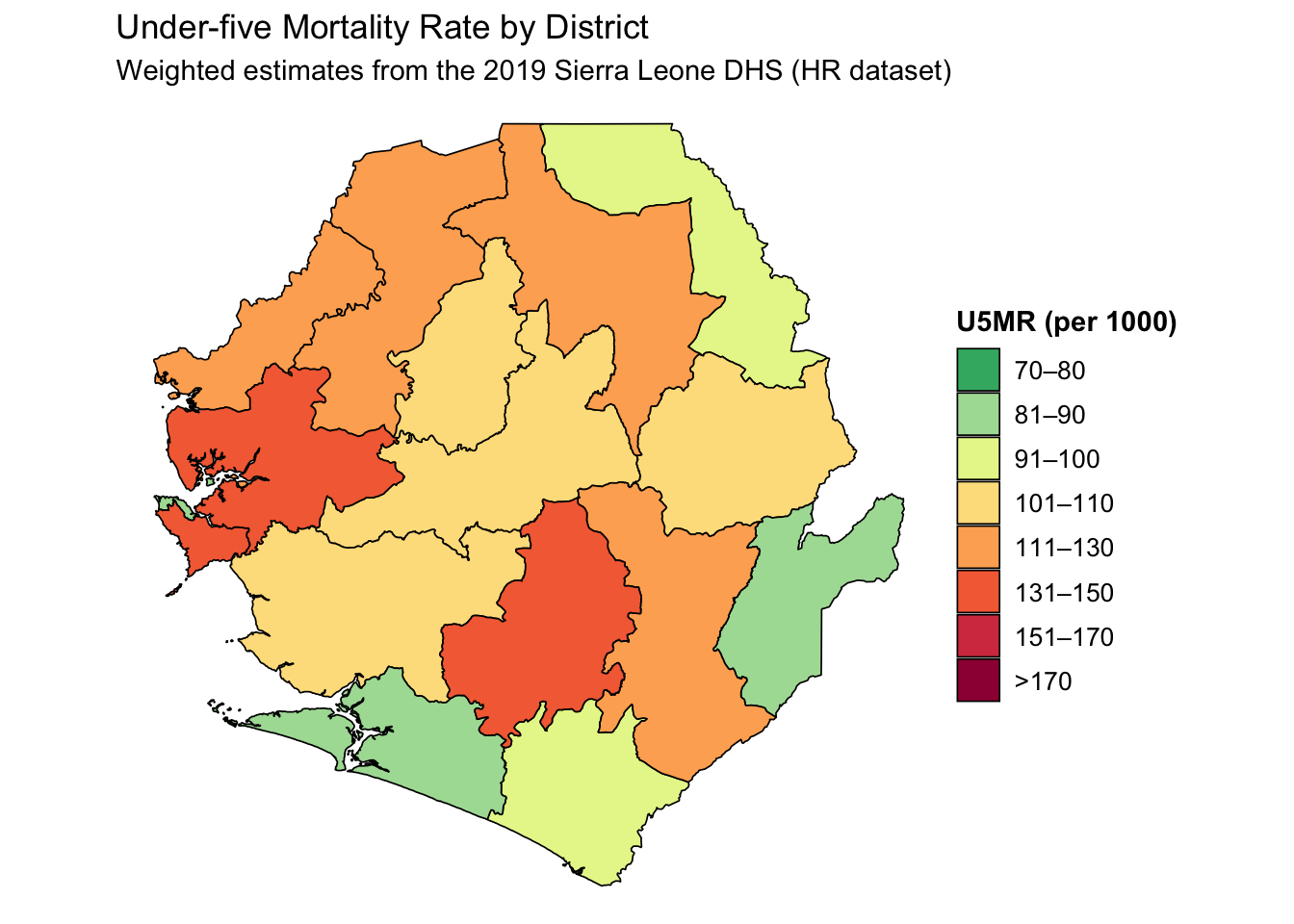
#===============================================================================
# Step 2.4: Plot U5MR at District Level
#===============================================================================
u5mr_final <- mort_sl2 |>
dplyr::left_join(
dplyr::select(sle_dhs_shp2, adm1, adm2),
by = c("adm1", "adm2")
) |>
dplyr::mutate(
prop_cat = cut(
mean_u5mr,
breaks = c(0, 80, 90, 100, 110, 130, 150, 170, Inf),
labels = c(
"70–80",
"81–90",
"91–100",
"101–110",
"111–130",
"131–150",
"151–170",
">170"
),
include.lowest = TRUE,
right = FALSE
)
)
# visualise the U5MR results
map_u5mr <- u5mr_final |>
ggplot2::ggplot() +
ggplot2::geom_sf(
ggplot2::aes(fill = prop_cat, geometry = geometry),
color = "black",
size = 0.3,
show.legend = TRUE
) +
ggplot2::scale_fill_manual(
name = "U5MR (per 1000)",
values = c(
">170" = "#9E0142",
"151–170" = "#D53E4F",
"131–150" = "#F46D43",
"111–130" = "#FDAE61",
"101–110" = "#FEE08B",
"91–100" = "#E6F598",
"81–90" = "#ABDDA4",
"70–80" = "#3CB371"
),
drop = FALSE
) +
ggplot2::labs(
title = "Under-five Mortality Rate by District",
subtitle = "Weighted estimates from the 2019 Sierra Leone DHS (HR dataset)"
) +
ggplot2::theme_void() +
ggplot2::theme(
legend.title = ggplot2::element_text(face = "bold"),
legend.text = ggplot2::element_text(size = 10)
)
map_u5mr
# save u5mr plot
ggplot2::ggsave(
  plot = map_u5mr,
  filename = here::here("03_output/3a_figures/u5mr_sle_adm2.png"),
  width = 12, height = 9, dpi = 300
)
#===============================================================================
# Step 2.5: Save Processed U5MR
#===============================================================================
# Define save directory
save_path <- here::here("1.6_health_systems/1.6a_dhs")
# Save final joined U5MR data
rio::export(
sle_dhs_shp2 |> sf::st_drop_geometry(),
here::here(save_path, "processed", "final_u5mr_sle_adm2.csv")
)
# Save final joined U5MR data with spatial data
rio::export(
sle_dhs_shp2,
here::here(save_path, "processed", "final_u5mr_sle_adm2.rds")
)
#===============================================================================
# End of Script
#===============================================================================