# installer `pacman` s'il n'est pas déjà installé
if (!requireNamespace("pacman", quietly = TRUE)) {
  install.packages("pacman")
}

# charger les paquets requis en utilisant pacman
pacman::p_load(
  sf,         # gestion des données shapefile
  dplyr,      # manipulation de données
  ggplot2,    # tracé
  here,       # gestion des chemins de fichiers
  stringr,    # manipulation de chaînes (par exemple, str_remove)
  cli,        # journalisation propre et messages de style CLI
  devtools    # pour la gestion des paquets
)

# sntutils a un certain nombre de fonctions d'aide utiles pour
# la gestion et le nettoyage des données
if (!requireNamespace("sntutils", quietly = TRUE)) {
  devtools::install_github("ahadi-analytics/sntutils")
}Gestion et personnalisation des shapefiles
Intermédiaire
Aperçu
Dans le contexte SNT, disposer d’un shapefile officiel, précis et à jour est important. Ces limites déterminent l’échelle à laquelle les analystes agrègent les données, calculent les indicateurs, appliquent les critères de ciblage et visualisent les résultats. Des shapefiles mal alignés ou incomplets peuvent introduire des erreurs graves, telles que des zones omises, des unités mal classées ou des cartes trompeuses, ce qui compromet à la fois la validité de l’analyse et son utilité pour la prise de décision.
TipEn savoir plus sur les données spatiales
Pour des informations générales sur les shapefiles et des liens vers tout le contenu sur les données spatiales dans la bibliothèque de code SNT, y compris les rasters et les données ponctuelles, veuillez consulter Aperçu des données spatiales.
Une bonne gestion des shapefiles, incluant le nettoyage des attributs, l’harmonisation des noms, la validation de la géométrie et la simplification de l’affichage, est nécessaire pour la cohérence spatiale, la reproductibilité et l’alignement avec les objectifs SNT. Une couche de limites validée sous-tend toutes les jointures, analyses et sorties dans le flux de travail SNT. Cette section présente les concepts de base des shapefiles et décrit les étapes clés pour les préparer et les personnaliser en vue de leur utilisation.
Cette page présente les étapes de base pour gérer et personnaliser les shapefiles en vue de leur utilisation dans le flux de travail SNT. Le shapefile de Sierra Leone préparé dans ces sections, ainsi que les concepts de visualisation et les connaissances spatiales introduits, sont utilisés dans le reste de la bibliothèque de code SNT pour soutenir toutes les étapes d’analyse et de cartographie.
ImportantGuide de référence fondamental
Cette page sert de référence fondamentale pour toutes les opérations spatiales dans la bibliothèque de code SNT. Une grande partie des pages d’analyse ultérieures, y compris celles qui téléchargent et traitent des données raster telles que la population, le climat et les estimations modélisées, s’appuient fortement sur les méthodes de gestion, de nettoyage et de dépannage des shapefiles présentées ici. Les techniques de validation de la géométrie, d’alignement du système de référence de coordonnées, d’agrégation des limites et de traitement des doublons sont des prérequis importants pour des jointures spatiales réussies et une analyse géographique précise tout au long du flux de travail SNT.
Il vaut la peine de s’assurer que le shapefile est capable de passer ces contrôles de validation dès le départ pour éviter tout problème par la suite. Mettez cette page en signet comme guide de référence auquel revenir lorsque vous rencontrez des problèmes de données spatiales dans les étapes d’analyse ultérieures.
NoteObjectifs
- Importer, inspecter et préparer des shapefiles et autres formats
- Valider et nettoyer les géométries pour garantir des jointures et des cartes précises
- Agréger ou personnaliser les limites administratives pour une analyse flexible
- Générer des empreintes de géométrie
- Enregistrer les fichiers shapefile nettoyés pour une utilisation ultérieure
Considérations pour la gestion et la personnalisation des shapefiles
Avant qu’un shapefile soit utilisé à quelque fin que ce soit, que ce soit pour joindre des données, visualiser des cartes, agréger des indicateurs ou exécuter une analyse spatiale, il doit être propre, valide et correctement structuré. Cette section décrit les principaux défis et les meilleures pratiques en matière de préparation des shapefiles qui guident la fiabilité de toutes les étapes en aval dans le flux de travail SNT. Ces étapes constituent la fondation de données sur laquelle repose une analyse SNT fiable.
Géométries valides et complètes
Les shapefiles doivent être géométriquement valides. Les problèmes possibles incluent :
- les artefacts spatiaux et les chevauchements dus à une mauvaise numérisation
- les polygones vides ou de surface nulle
- les géométries multiparties ou les trous qui affectent la logique de confinement.
Les géométries invalides peuvent silencieusement casser les jointures ou mal placer les entités. Dans les flux de travail SNT, cela peut entraîner des zones manquantes dans les cartes de couverture ou des grappes non appariées dans l’analyse des données d’enquête. Il est toujours important d’identifier les géométries invalides, de les signaler et de les corriger lorsque cela est possible.
Garantir des polygones uniques
Chaque unité du shapefile doit représenter une zone géographique unique et distincte. Les polygones en double, causés par des erreurs de numérisation ou des enregistrements répétés par erreur, peuvent entraîner des jointures incorrectes, un double comptage dans les agrégations et une confusion dans la cartographie.
Pourquoi c’est important : les entités en double avec le même nom ou le même ID peuvent :
- Fausser les statistiques récapitulatives
- Conduire à des correspondances incorrectes lors de la jointure de plusieurs shapefiles
- Créer des visualisations ou des cartes trompeuses
Problèmes possibles à résoudre :
Géométries en double (polygones ou autre géométrie) avec des ID identiques ou répétés
Plusieurs enregistrements représentant la même unité
Exemple : si deux entités portent toutes deux le nom « Bumpe Ngao » et couvrent la même zone, les estimations de population peuvent être comptées deux fois lors de l’extraction zonale ou des calculs d’incidence. L’un des doublons doit être supprimé avant d’utiliser le shapefile.
Nous pouvons utiliser des outils géospatiaux pour détecter et résoudre les doublons, tels que signaler les noms ou les ID répétés, comparer les géométries pour l’égalité ou dissoudre les entités par codes administratifs. Nous allons démontrer plusieurs exemples dans la section Étape par étape ci-dessous.
Systèmes de référence de coordonnées (CRS)
Pour que les jointures spatiales fonctionnent correctement, les deux fichiers de données spatiales doivent partager le même CRS. Une non-concordance peut faire en sorte que les points tombent en dehors de leurs vrais polygones, même si les coordonnées sont correctes. Confirmez toujours que les deux jeux de données utilisent un CRS commun et approprié, car les non-concordances peuvent entraîner un mauvais alignement et des résultats incorrects. En général, WGS84 (EPSG:4326) est utilisé. Pour plus d’informations sur le CRS, veuillez consulter Aperçu des données spatiales.
Agréger ou reconstruire les niveaux administratifs
Avant de commencer toute analyse, les analystes doivent demander tous les shapefiles officiels au niveau d’unité d’analyse requis et à tous les niveaux administratifs supérieurs. Par exemple, si l’unité choisie est adm2, nous devons également obtenir le shapefile adm1 officiel. Ceci est important pour harmoniser les données entre les niveaux et pour produire des cartes SNT qui incluent le contexte national et régional et sont faciles à interpréter.
En pratique, nous pouvons constater que le shapefile pour l’unité d’analyse prévue est manquant ou incomplet. Par exemple, nous pourrions avoir des données à adm2 mais seulement un shapefile complet pour adm3. Dans de tels cas, nous pouvons agréger des polygones à partir d’un shapefile plus granulaire en utilisant un identifiant partagé pour reconstruire les limites de niveau supérieur.
- Les polygones
adm3peuvent être regroupés et dissous par un nom ou un codeadm2commun pour recréer les limitesadm2. La même approche s’applique aux limitesadm1. - Cette technique est utilisée dans le SNT lors du reporting à des niveaux plus larges (par exemple, provinces ou régions) ou lors de la visualisation de cartes nationales avec une résolution cohérente, si des shapefiles dédiés à l’unité administrative plus grande ne sont pas disponibles.
Exemple : en Sierra Leone, si seules les limites
adm3sont disponibles, nous pouvons regrouper les unitésadm3par leur nom de district et fusionner leurs géométries. Cela reconstruit un shapefile de niveauadm2qui correspond aux données et permet une cartographie et une agrégation précises.
Ce processus garantit que la structure du shapefile s’aligne sur le niveau des indicateurs et prend en charge des jointures, des visualisations et des rapports propres entre les niveaux administratifs.
Agrégation partielle pour une résolution flexible
Dans certains cas, il peut être bénéfique de représenter différentes parties du pays à différents niveaux administratifs au sein du même shapefile. Par exemple, une analyse SNT peut nécessiter des détails adm3 pour les zones d’élimination, tandis que le reste du pays peut être visualisé et analysé à adm2.
Cette stratégie est particulièrement utile lorsque les interventions ou les décisions programmatiques nécessitent plus de granularité dans certaines zones que dans d’autres. Elle offre un moyen pratique d’équilibrer les détails et l’utilisabilité dans les cartes et l’analyse tout en garantissant l’alignement avec les priorités spécifiques au pays et les besoins opérationnels. Cette approche nous permet de conserver des limites détaillées dans certaines zones tout en utilisant des limites d’unités plus grandes ailleurs.
NoteGestion des niveaux administratifs mixtes au sein d’un pays
Dans certains exercices SNT, les pays choisissent d’utiliser différents niveaux administratifs dans différentes régions, par exemple, adm3 pour les zones urbaines et adm2 pour les zones rurales. Cela reflète les réalités opérationnelles, la disponibilité des données ou les besoins de planification.
Pour soutenir cette configuration hybride, nous pouvons découper chaque shapefile dans sa région pertinente puis les fusionner en une seule couche de limites. Avec un alignement approprié des géométries et des attributs, cette structure permet une analyse spatiale flexible et sensible au contexte. Les techniques nécessaires pour ce faire sont couvertes sur cette page.
Suivi des changements de limites
Les limites administratives peuvent évoluer au fil du temps, par le biais de redécoupages, de renommages ou de reclassifications. Dans le SNT, il est important de détecter ces changements pour garantir la cohérence géographique pour l’analyse de séries chronologiques ou de tendances, et pour s’assurer que les données historiques sont cartographiées et interprétées correctement.
Bien que la visualisation et la comparaison de différentes versions d’un shapefile à l’œil nu soit un moyen simple de rechercher des différences visibles, il est également possible de détecter les changements de manière plus systématique et rigoureuse. Une façon de le faire est de générer une empreinte de géométrie, un identifiant unique basé sur les coordonnées d’un polygone. Si une forme change, son empreinte changera. Si seul le nom ou le code change mais que la géométrie reste la même, l’empreinte reste stable, ce qui facilite la détection des renommages ou la confirmation de la continuité spatiale.
Exemple : si la géométrie du district de Kambia est inchangée mais renommée entre les versions, son empreinte reste la même. Si la forme est redessinée, l’empreinte sera différente, la signalant pour examen.
Cette approche prend en charge le contrôle de version, la cohérence longitudinale et les flux de travail spatiaux reproductibles. Les méthodes de calcul et de comparaison des empreintes sont couvertes plus loin dans cette section.
Étape par étape
Dans cette section, nous parcourons les étapes importantes pour charger, gérer, dépanner et personnaliser les données shapefile.
L’exemple utilise des shapefiles de limites administratives de Sierra Leone, en se concentrant sur les niveaux chefferie (adm3) et district (adm2). Les principes peuvent être appliqués aux shapefiles de n’importe quel pays.
Pour passer l’explication étape par étape, accédez au code complet à la fin de cette page.
Étape 1 : Installer et charger les paquets
Tout d’abord, installez et/ou chargez les paquets nécessaires pour gérer les données spatiales, la manipulation des données et la visualisation. Ces bibliothèques fournissent des fonctions nécessaires pour travailler avec des données spatiales.
Le paquet sf est particulièrement important car il met en œuvre des normes de fonctionnalités simples pour gérer les données vectorielles géographiques dans R.
Pour adapter le code :
- Ne modifiez rien dans le code ci-dessus.
WarningInstallation requise dans le terminal
Installez les paquets dans votre terminal s’ils ne sont pas déjà installés. Si vous avez besoin d’aide pour installer les paquets, consultez la page Bien démarrer.
Une fois les paquets installés, chargez les paquets pertinents et définissez quelques fonctions d’aide pour les graphiques, les empreintes de géométrie et la validation des géométries.
from pathlib import Path

import geopandas as gpd            # gestion des données vectorielles spatiales
import matplotlib.colors as mcolors
import matplotlib.patches as mpatches
import matplotlib.pyplot as plt    # visualisation
import numpy as np                 # logique conditionnelle et tableaux
import pandas as pd                # manipulation de données
import xxhash                      # hachage rapide et stable
from pyprojroot import here        # chemins relatifs à la racine du projet
from shapely import make_valid
from shapely.geometry import GeometryCollection, MultiPolygon, Polygon
from shapely.ops import unary_union
from shapely.validation import explain_validity


def cli_info(message):
    """Afficher un message simple similaire à cli::cli_alert_info()."""
    print(f"INFO: {message}")


def cli_header(message):
    """Afficher un en-tête simple similaire à cli::cli_h1()/cli_h2()."""
    print(f"\n{message}")


def cli_success(message):
    """Afficher un message de succès similaire à cli::cli_alert_success()."""
    print(f"SUCCESS: {message}")


def cli_warning(message):
    """Afficher un message d'avertissement similaire à cli::cli_alert_warning()."""
    print(f"WARNING: {message}")


def cli_danger(message):
    """Afficher un message d'erreur similaire à cli::cli_alert_danger()."""
    print(f"ERROR: {message}")


def sf_colors(n=10):
    """Reproduire sf::sf.colors(..., categorical = TRUE) avec matplotlib."""
    palette_name = "Set2" if n <= 8 else "Set3"
    palette = [mcolors.to_hex(color) for color in plt.get_cmap(palette_name).colors]
    return [palette[i % len(palette)] for i in range(n)]


R_COLOR_MAP = {
    "grey10": "#1a1a1a",
    "gray10": "#1a1a1a",
    "grey30": "#4d4d4d",
    "gray30": "#4d4d4d",
    "grey90": "#e5e5e5",
    "gray90": "#e5e5e5",
}


def r_color(color):
    """Traduire les noms de couleurs R courants en couleurs matplotlib."""
    return R_COLOR_MAP.get(color, color)


def geometry_wkb(geom):
    """Retourner les octets WKB pour les vérifications de doublons exacts."""
    if geom is None:
        return None
    return geom.wkb


def geometry_hash(geom, algo="xxhash32"):
    """Créer une empreinte de géométrie basée sur WKB."""
    if geom is None:
        return None
    payload = geom.wkb
    if algo == "xxhash32":
        return xxhash.xxh32(payload).hexdigest()
    if algo == "xxhash64":
        return xxhash.xxh64(payload).hexdigest()
    raise ValueError("Seuls xxhash32 et xxhash64 sont implémentés ici.")


def polygonal_part(geom):
    """Conserver la partie polygonale après make_valid()."""
    if geom is None or geom.is_empty:
        return geom
    if isinstance(geom, (Polygon, MultiPolygon)):
        return geom
    if isinstance(geom, GeometryCollection):
        pieces = [
            part for part in geom.geoms
            if isinstance(part, (Polygon, MultiPolygon))
        ]
        return unary_union(pieces) if pieces else geom
    return geom


def make_valid_polygonal(geom):
    """Équivalent Python de sf::st_make_valid() pour les couches polygonales."""
    return polygonal_part(make_valid(geom))


def as_geodataframe(data, crs=None):
    """Convertir GeoDataFrame, GeoSeries ou liste de géométries en GeoDataFrame."""
    if isinstance(data, gpd.GeoDataFrame):
        return data
    if isinstance(data, gpd.GeoSeries):
        return gpd.GeoDataFrame(geometry=data, crs=data.crs)
    return gpd.GeoDataFrame(geometry=gpd.GeoSeries(data), crs=crs)


def plot_sf_like(
    data,
    ax=None,
    colors=None,
    border="grey10",
    linewidth=0.35,
    title=None,
    title_size=12,
):
    """Tracer une carte avec un style proche du tracé sf de base dans R."""
    gdf = as_geodataframe(data)
    if ax is None:
        _, ax = plt.subplots()

    if colors is None:
        colors = sf_colors(len(gdf))
    elif isinstance(colors, str):
        colors = r_color(colors)
    else:
        colors = [r_color(colors[i % len(colors)]) for i in range(len(gdf))]

    gdf.plot(
        ax=ax,
        color=colors,
        edgecolor=r_color(border) if border else None,
        linewidth=linewidth,
    )
    ax.set_title(title or "", fontsize=title_size)
    ax.set_axis_off()
    ax.set_aspect("equal")
    return ax
Pour adapter le code :
- Ne modifiez pas ce bloc d’importation sauf si votre environnement Python utilise un autre outil pour les chemins de projet ou si une importation échoue.
- Conservez les fonctions d’aide dans ce premier bloc Python. Les sections de visualisation, d’empreinte de géométrie et d’exportation ci-dessous en dépendent.
Étape 2 : Charger et préparer les shapefiles
Étape 2.1 : Charger et examiner les données
Importez les deux jeux de données et examinez leur structure pour identifier les clés de jointure appropriées. Cette étape importante garantit la compréhension des données avant de tenter de les fusionner.
Nous commençons par charger le shapefile de Sierra Leone et sélectionner les niveaux administratifs pertinents pour l’analyse. Une nouvelle colonne pour adm0 (nom du pays) est ajoutée, et les champs d’unité administrative sont renommés en étiquettes standard adm1, adm2 et adm3 pour la cohérence dans le flux de travail SNT.
# configurer le chemin spatial
spat_path <- here::here(
"01_data", "1.1_foundational", "1.1a_admin_boundaries"
)
# importer le shapefile
shp_adm3 <- sf::read_sf(
here::here(spat_path, "raw", "Chiefdom2021.shp")
) |>
dplyr::mutate(adm0 = "SIERRA LEONE") |>
dplyr::select(
# sélectionner les colonnes pertinentes et renommer selon la nomenclature standard
adm0,
adm1 = FIRST_REGI,
adm2 = FIRST_DNAM,
adm3 = FIRST_CHIE
) |>
# garantir que la sortie reste un objet sf valide pour une utilisation en aval
sf::st_as_sf()
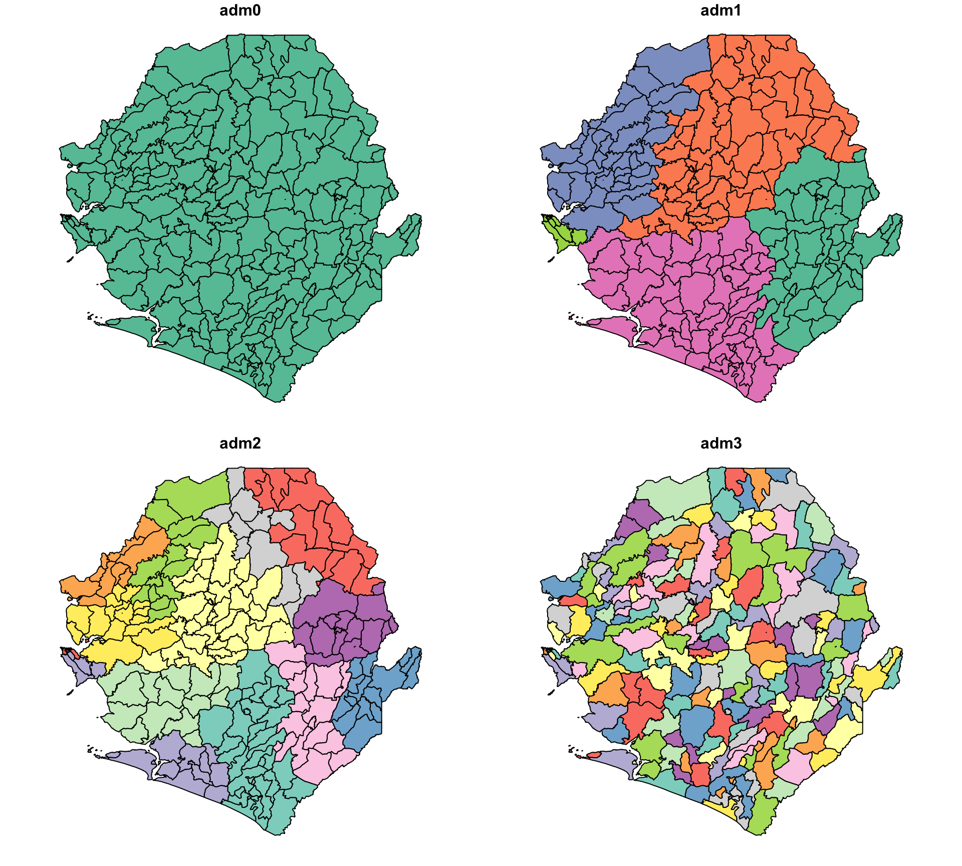
# vérifier la sortie par cartographie
plot(shp_adm3)
NoteSortie
Pour adapter le code :
Le code ci-dessous montre comment modifier le processus de chargement lorsque vous travaillez avec d’autres formats vectoriels spatiaux. Tous ces exemples utilisent sf::read_sf(), qui prend en charge plusieurs formats via GDAL.
GeoJSON : si le fichier de limites est au format GeoJSON, mettez simplement à jour l’extension de fichier
GeoPackage (.gpkg) : pour les fichiers GeoPackage, nous devons spécifier à la fois le fichier et le nom de la couche :
ℹ️ Utilisez
sf::st_layers("boundary.gpkg")pour lister toutes les couches disponibles dans le fichier.
File Geodatabase (.gdb) : pour les fichiers Geodatabase, nous devons spécifier à la fois le fichier et le nom de la couche :
Une fois importé, le reste du pipeline de traitement (mutate(), select(), st_set_crs(), etc.) reste le même.
Adaptations supplémentaires :
- Ligne 2 : modifiez le chemin
here::here()pour correspondre à la structure de dossiers - Ligne 5 : si vous travaillez avec un shapefile à un niveau d’unité administrative différent, changez le nom de variable pour l’objet spatial de
shp_adm3. Par exemple, si vous travaillez à adm2,shp_adm2serait plus approprié. - Lignes 11–14 : mettez à jour les noms de colonnes administratives (
adm0,adm1,adm2,adm3) pour refléter le jeu de données. Par exemple, si le shapefile ne contient pas de niveau adm3, supprimez la ligne adm3.
# configurer le chemin spatial
spat_path = here("01_data/1.1_foundational/1.1a_admin_boundaries")
# importer le shapefile
shp_adm3 = (
gpd.read_file(Path(spat_path) / "raw" / "Chiefdom2021.shp")
.assign(adm0="SIERRA LEONE")
.rename(columns={
"FIRST_REGI": "adm1",
"FIRST_DNAM": "adm2",
"FIRST_CHIE": "adm3",
})
[["adm0", "adm1", "adm2", "adm3", "geometry"]]
)
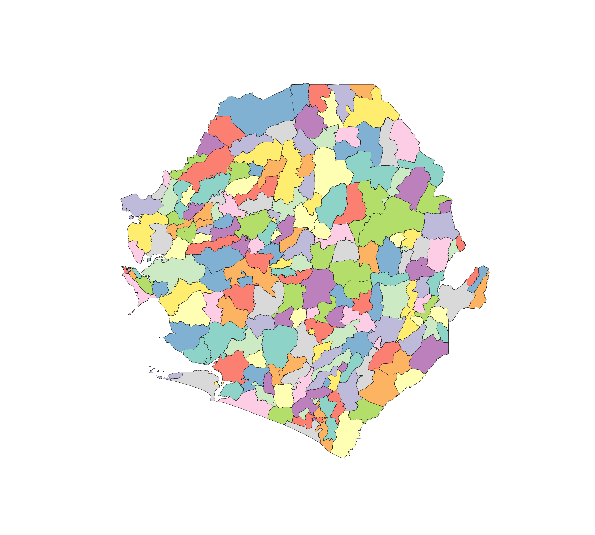
# vérifier la sortie par cartographie
ax = plot_sf_like(shp_adm3, title="")
plt.show()
NoteSortie
GeoJSON : si le fichier de limites est au format GeoJSON, mettez simplement à jour l’extension de fichier
GeoPackage (.gpkg) : pour les fichiers GeoPackage, nous devons spécifier à la fois le fichier et le nom de la couche :
Utilisez
gpd.list_layers("boundary.gpkg")pour lister toutes les couches disponibles dans le fichier.
File Geodatabase (.gdb) : pour les fichiers Geodatabase, nous devons spécifier à la fois le fichier et le nom de la couche :
Pour adapter le code :
- Ligne 2 : modifiez le chemin
here()pour correspondre à la structure de dossiers. - Ligne 5 : si vous travaillez avec un shapefile à un autre niveau administratif, changez le nom de variable de
shp_adm3, par exemple enshp_adm2. - Lignes 10–14 : mettez à jour les noms de colonnes administratives (
adm0,adm1,adm2,adm3) pour refléter le jeu de données. Si le shapefile ne contient pas de niveau adm3, supprimez la ligneadm3. - Pour les entrées GeoJSON, GeoPackage et Geodatabase, conservez les mêmes étapes de nettoyage en aval après
gpd.read_file().
Les cartes R et Python sont différentes parce que le comportement par défaut des fonctions de tracé diffère : plot() sur un objet sf en R dessine un panneau par attribut, tandis que GeoDataFrame.plot() en Python rend une seule carte. Les données sous-jacentes sont identiques.
Étape 2.2 : Vérifier et transformer le CRS
Une fois chargé, il est important de s’assurer que le shapefile est dans le système de référence de coordonnées (CRS) approprié.
Ci-dessous, nous vérifions le CRS actuel du shapefile et, si nécessaire, le transformons en un système de référence géographique cohérent, pour garantir que toutes les couches s’alignent correctement et seront compatibles avec d’autres jeux de données spatiaux que nous pourrions utiliser.
Le shapefile de Sierra Leone est déjà en WGS84 (EPSG:4326), donc normalement nous n’aurions pas besoin de changer le CRS. Cependant, à des fins de démonstration, nous fournissons un exemple de comment transformer le CRS (en Equal Earth (EPSG:6933)).
cli::cli_h2("Vérifier et attribuer la CRS d'origine pour shp_adm3")
shp_adm3 <- sf::st_set_crs(shp_adm3, 4326)
cli::cli_alert_info("CRS d'origine : {sf::st_crs(shp_adm3)$input}")

# transformer en nouvelle CRS (par exemple, Equal Earth - EPSG:6933)
shp_adm3_diff_crs <- sf::st_transform(shp_adm3, 6933)

cli::cli_h2("Vérifier la CRS après transformation")
cli::cli_alert_info("Nouvelle CRS : {sf::st_crs(shp_adm3_diff_crs)$input}")Pour adapter le code :
- Lignes 1–2 : ne changez rien sauf si vous utilisez une variable différente pour l’objet shapefile (par exemple,
shp_adm2) ou avez besoin d’un CRS différent. - Ligne 2 : utilisez
st_set_crs()uniquement si le shapefile manque de CRS mais que nous sommes certains de ce qu’il devrait être. Pour reprojeter la géométrie, utilisez toujoursst_transform(). - Ligne 6 : pour utiliser une autre projection, mettez simplement à jour le code EPSG dans
st_transform(), par exemple à 4326 pour le CRS WGS84 généralement utilisé dans le SNT, si le shapefile d’origine avait un CRS différent. - Si le shapefile était déjà dans le bon CRS, les lignes 6 et suivantes peuvent être supprimées.
cli_header("Vérifier et attribuer la CRS d'origine pour shp_adm3")
shp_adm3 = shp_adm3.set_crs(epsg=4326, allow_override=True)
cli_info(f"CRS d'origine : {shp_adm3.crs}")

# transformer en nouvelle CRS (par exemple, Equal Earth - EPSG:6933)
shp_adm3_diff_crs = shp_adm3.to_crs(epsg=6933)

cli_header("Vérifier la CRS après transformation")
cli_info(f"Nouvelle CRS : {shp_adm3_diff_crs.crs}")Pour adapter le code :
- Lignes 2–3 : remplacez
shp_adm3par le nom de variable pour l’objet spatial pertinent. - Ligne 3 : utilisez
.set_crs()uniquement si le shapefile manque de CRS et que nous sommes certains de ce qu’il devrait être. Pour reprojeter la géométrie, utilisez toujours.to_crs(). - Ligne 7 : pour utiliser une autre projection, mettez à jour le code EPSG dans
.to_crs(epsg=...). - Si le shapefile était déjà dans le bon CRS, les lignes 6 et suivantes peuvent être supprimées.
Étape 3 : Validation de la géométrie
Étape 3.1 : Vérifier et corriger la validité de la géométrie
Les géométries invalides, comme les chevauchements, les trous ou les formes brisées, peuvent faire échouer les jointures ou désaligner les cartes. Ces problèmes peuvent passer inaperçus mais conduisent finalement à des zones manquantes ou des sorties incorrectes. Avant de faire des jointures, vérifiez toujours que le shapefile est valide.
# vérifier la validité de la géométrie
shp_adm3_inv <- shp_adm3 |>
  dplyr::mutate(
    valid = sf::st_is_valid(geometry),
    invalid_reason = sf::st_is_valid(geometry, reason = TRUE),
    invalid_reason = stringr::str_remove(invalid_reason, "\\[.*")
  )

# obtenir la liste des adm3 invalides
invalid_df <- shp_adm3_inv |>
  dplyr::filter(!valid) |>
  sf::st_drop_geometry() |>
  dplyr::select(adm0, adm1, adm2, adm3, invalid_reason)

# afficher les lignes invalides (le cas échéant)
invalid_dfPour adapter le code :
- Lignes 2, 10 et 13 : remplacez
shp_adm3par le nom de variable pour l’objet spatial pertinent, tel queshp_adm2.
# vérifier la validité de la géométrie
shp_adm3_inv = shp_adm3.copy()
shp_adm3_inv["valid"] = shp_adm3_inv.geometry.is_valid
shp_adm3_inv["invalid_reason"] = (
    shp_adm3_inv.geometry.apply(explain_validity)
    .str.replace(r"\[.*", "", regex=True)
    .str.strip()
)

# obtenir la liste des adm3 invalides
invalid_df = (
    shp_adm3_inv.loc[~shp_adm3_inv["valid"], [
        "adm0", "adm1", "adm2", "adm3", "invalid_reason"
    ]]
    .reset_index(drop=True)
)

# afficher les lignes invalides (le cas échéant)
invalid_dfPour adapter le code :
- Lignes 2, 5 et 13 : remplacez
shp_adm3par le nom de variable pour l’objet spatial pertinent, tel queshp_adm2. - Ligne 15 : mettez à jour les colonnes administratives sélectionnées si le shapefile utilise des noms de champs différents.
Deux chefferies, Niawa et Wara Wara Yagala, ont des géométries invalides en raison d’auto-intersections d’anneaux, où les bords de polygones se croisent ou rebouclent sur eux-mêmes (voir ce guide pour les raisons courantes de géométrie invalide). Ces problèmes ont tendance à résulter d’erreurs de numérisation ou de limites trop complexes et peuvent perturber les jointures spatiales et les visualisations. Il est important de les identifier et de les corriger avant un traitement ultérieur.
Nous conserverons invalid_df pour référence, car il contient les chefferies avec des problèmes non résolus pour un examen manuel potentiel ou une référence future, puis nous procéderons pour rendre toutes les géométries dans shp_adm3 valides.
# corriger les problèmes de géométrie connus
# (par exemple, auto-intersections, anneaux non fermés)
shp_adm3 <- shp_adm3 |>
  sf::st_make_valid()

# revérifier et signaler les géométries invalides restantes
n_invalid <- shp_adm3 |>
  dplyr::mutate(valid = sf::st_is_valid(geometry)) |>
  dplyr::filter(!valid) |>
  nrow()

cli::cli_alert_info("Géométries invalides restantes : {n_invalid}")Pour adapter le code :
- Lignes 3 et 7 : remplacez
shp_adm3par l’objet spatial pertinent, tel queshp_adm2.
# corriger les problèmes de géométrie connus
# (par exemple, auto-intersections, anneaux non fermés)
shp_adm3 = shp_adm3.copy()
shp_adm3["geometry"] = shp_adm3.geometry.apply(make_valid_polygonal)

# revérifier et signaler les géométries invalides restantes
n_invalid = int((~shp_adm3.geometry.is_valid).sum())

cli_info(f"Géométries invalides restantes : {n_invalid}")Pour adapter le code :
- Lignes 3 et 7 : remplacez
shp_adm3par l’objet spatial pertinent, tel queshp_adm2. - Conservez
make_valid_polygonal()du bloc de configuration afin que les collections de géométries soient reconverties en sortie polygonale lorsque c’est possible.
Toutes les géométries sont maintenant valides et sûres pour les opérations spatiales futures.
Étape 3.2 : Vérifier les polygones en double
Chaque polygone doit représenter une unité géographique unique. Les formes en double, qu’il s’agisse de copies exactes ou de plusieurs enregistrements pour la même zone, peuvent entraîner un double comptage, des erreurs de jointure et des résumés trompeurs. Vérifiez toujours et supprimez les doublons avant de continuer. Ci-dessous, nous décrivons des vérifications et des corrections simples en utilisant des approches standard.
Pour adapter le code :
- Lignes 2 et 6 : remplacez
shp_adm3par l’objet spatial pertinent, tel queshp_adm2.
Pour adapter le code :
- Lignes 2 et 6 : remplacez
shp_adm3par l’objet spatial pertinent, tel queshp_adm2. - Conservez la fonction d’aide
geometry_wkb()pour les vérifications de doublons de géométrie exacts, car elle reflète le rôle desf::st_as_binary(geometry).
Les résultats montrent 5 géométries non uniques. Il est important de les enquêter et de les résoudre avant de procéder à l’analyse ou à l’intégration. Nous utilisons la vérification ci-dessous pour identifier les doublons en fonction des attributs et de la géométrie. Il est utile de distinguer entre :
- Doublons de ligne complète : mêmes attributs et même géométrie.
- Doublons de géométrie uniquement : formes identiques avec des étiquettes différentes.
# vérifier les doublons de ligne complète
dups_full <- shp_adm3 |>
dplyr::group_by(dplyr::across(dplyr::everything())) |>
dplyr::filter(dplyr::n() > 1)
# vérifier les doublons de géométrie uniquement
dups_geom <- shp_adm3 |>
dplyr::mutate(geom_hash = sntutils::vdigest(geometry)) |>
dplyr::add_count(geom_hash, name = "n_geom") |>
dplyr::filter(n_geom > 1)
# afficher les résultats
cli::cli_h1("Vérification des doublons de ligne complète")
dups_full |> sf::st_drop_geometry()
cli::cli_h1("Vérification des doublons de géométrie uniquement")
dups_geom |> sf::st_drop_geometry()Pour adapter le code :
- Lignes 2, 7, 14 et 17 : remplacez
shp_adm3par l’objet spatial pertinent, tel queshp_adm2. - Assurez-vous que la colonne de géométrie est nommée geometry (comme c’est le cas avec
sf::read_sf()).
# vérifier les doublons de ligne complète
shp_adm3_for_dups = shp_adm3.assign(
geometry_wkb=shp_adm3.geometry.apply(geometry_wkb)
)
dups_full = (
shp_adm3_for_dups
.loc[
shp_adm3_for_dups.duplicated(
subset=["adm0", "adm1", "adm2", "adm3", "geometry_wkb"],
keep=False
)
]
.drop(columns="geometry_wkb")
)
# vérifier les doublons de géométrie uniquement
dups_geom = (
shp_adm3.assign(geom_hash=shp_adm3.geometry.apply(geometry_hash))
.assign(n_geom=lambda x: x.groupby("geom_hash")["geom_hash"].transform("size"))
.loc[lambda x: x["n_geom"] > 1]
)
# afficher les résultats
cli_header("Vérification des doublons de ligne complète")
dups_full.drop(columns="geometry")
cli_header("Vérification des doublons de géométrie uniquement")
dups_geom.drop(columns="geometry")Pour adapter le code :
- Lignes 2, 7, 18 et 22 : remplacez
shp_adm3par l’objet spatial pertinent, tel queshp_adm2. - Lignes 9–10 : mettez à jour les colonnes d’attributs utilisées pour vérifier les doublons de ligne complète si le shapefile utilise d’autres noms administratifs.
- Assurez-vous que la colonne de géométrie est nommée
geometry, comme c’est le cas avecgpd.read_file().
Dans cet exemple :
DEAetJAHNapparaissent chacun deux fois avec des attributs et une géométrie identiques, indiquant des doublons de ligne complète. Ceux-ci sont probablement accidentels (par exemple, créés lors de la fusion ou de la liaison) et peuvent être supprimés en toute sécurité en utilisant une étape de déduplication appropriée au logiciel ou au langage en cours d’utilisation.MALEMAetDUPLICATE LABELpartagent la même géométrie mais ont des noms différents. Cela suggère un problème d’étiquetage ou de nommage, pas un problème avec le shapefile lui-même. Ces cas peuvent refléter une convention administrative ou une jointure non correspondante, plutôt qu’une erreur spatiale.
TipUtilisez les empreintes de géométrie pour détecter les changements de géométrie
Nous utilisons le hachage de géométrie pour attribuer un ID unique à chaque forme, ce qui facilite la détection et la comparaison des changements entre les versions de shapefile. Voir l’étape 6 pour plus de détails.
Étape 3.3 : Résoudre les polygones en double
Ensuite, nous allons résoudre les polygones en double dans notre shapefile. Nous supprimerons d’abord les doublons de ligne complète. Ensuite, pour les doublons de géométrie uniquement, nous supprimerons une version. Dans cet exemple, nous supprimerons le polygone avec le nom adm3 DUPLICATE LABEL. Enfin, nous vérifierons à nouveau les doublons de géométrie pour nous assurer que tous les doublons sont maintenant résolus.
ImportantConsultez l’équipe SNT
Si les doublons ne sont pas clairement redondants ou reflètent plus que de simples problèmes de saisie de données, consultez l’équipe SNT avant de prendre des décisions de réconciliation. Certains cas peuvent impliquer des unités opérationnelles qui se chevauchent, des conventions de nommage héritées ou des doublons intentionnels utilisés dans la planification. Ne supprimez rien à moins que l’objectif de la duplication ne soit compris.
Documentez toujours clairement les étapes de nettoyage, afin que l’équipe SNT soit au courant de toute modification et puisse retracer le processus si nécessaire.
# supprimer les doublons de ligne complète
shp_adm3 <- shp_adm3 |>
dplyr::distinct()
# si nécessaire, supprimer les doublons de géométrie uniquement connus en filtrant sur les étiquettes
# supprimer l'étiquette intentionnellement dupliquée
shp_adm3 <- shp_adm3 |>
dplyr::filter(adm3 != "DUPLICATE LABEL")
# vérifier à nouveau après nettoyage
# vérifier les doublons de géométrie uniquement dans shp_adm3
shp_adm3_dup <- shp_adm3 |>
dplyr::mutate(dup_geom = duplicated(sf::st_as_binary(geometry))) |>
dplyr::filter(dup_geom == TRUE)
cli::cli_alert_info(
"Nombre de géométries en double dans shp_adm3 : {nrow(shp_adm3_dup)}"
)Pour adapter le code :
- Lignes 2, 7, 12 et 16 : remplacez
shp_adm3par l’objet spatial pertinent, tel queshp_adm2. - Ligne 8 : mettez à jour la colonne utilisée dans
filter()(par exemple,adm3,facility_nameoudistrict_name) pour correspondre à la convention de nommage du jeu de données. - Ligne 2 : utilisez
dplyr::distinct()pour supprimer les lignes en double exactes (mêmes attributs et géométrie). - Ligne 8 : utilisez
dplyr::filter()pour supprimer les doublons connus basés sur les étiquettes en passant le nom de l’étiquette à supprimer (par exemple, lignes avecDUPLICATE LABEL).
# supprimer les doublons de ligne complète
shp_adm3 = (
shp_adm3.assign(geometry_wkb=shp_adm3.geometry.apply(geometry_wkb))
.drop_duplicates(
subset=["adm0", "adm1", "adm2", "adm3", "geometry_wkb"]
)
.drop(columns="geometry_wkb")
)
shp_adm3 = gpd.GeoDataFrame(shp_adm3, geometry="geometry", crs=shp_adm3.crs)
# si nécessaire, supprimer les doublons de géométrie uniquement connus en filtrant sur les étiquettes
# supprimer l'étiquette intentionnellement dupliquée
shp_adm3 = shp_adm3.loc[shp_adm3["adm3"] != "DUPLICATE LABEL"].copy()
# vérifier à nouveau après nettoyage
# vérifier les doublons de géométrie uniquement dans shp_adm3
shp_adm3_dup = (
shp_adm3.assign(
dup_geom=shp_adm3.geometry.apply(geometry_wkb).duplicated()
)
.loc[lambda x: x["dup_geom"]]
)
cli_info(f"Nombre de géométries en double dans shp_adm3 : {len(shp_adm3_dup)}")Pour adapter le code :
- Lignes 2, 13, 17 et 21 : remplacez
shp_adm3par l’objet spatial pertinent, tel queshp_adm2. - Lignes 5–6 : mettez à jour les colonnes de déduplication si le shapefile utilise d’autres noms administratifs.
- Ligne 14 : mettez à jour la colonne et l’étiquette utilisées pour supprimer les doublons connus de géométrie uniquement.
- Supprimez les doublons de géométrie uniquement après avoir confirmé quelle étiquette ou quel enregistrement doit être supprimé.
Les résultats montrent que les opérations ont fonctionné, car le jeu de données n’a plus de doublons de ligne complète ou de géométrie uniquement. Le jeu de données ne contient maintenant que des géométries uniques et valides.
TipVérifier les versions de limites historiques
Dans certains cas, les shapefiles ou les géodatabases peuvent inclure plusieurs versions des mêmes limites, chacune associée à des métadonnées indiquant quand cette limite était en vigueur (par exemple, start_date, end_date).
Vérifiez toujours la table d’attributs et les métadonnées pour les champs liés à la date. Si le jeu de données inclut des versions historiques, nous devrons peut-être filtrer pour obtenir les limites les plus récentes, telles que :
En Python, utilisez la même condition avec le filtrage pandas/geopandas :
🔎 Si vous n’êtes pas sûr de la façon dont les limites ont été versionnées ou étiquetées, consultez l’équipe SNT ou le propriétaire des données avant de continuer.
Étape 3.4 : Vérifier les trous topologiques et les fines bandes
Même lorsque les polygones individuels sont valides, la couche de limites dans son ensemble peut encore avoir des trous entre les unités voisines ou de fines bandes où les polygones adjacents se chevauchent. Ces artefacts sont généralement des erreurs de numérisation et sont difficiles à repérer visuellement, mais ils causent une perte de données silencieuse dans les flux de travail SNT :
- Les trous signifient que certains pixels d’un raster (population, climat, estimations modélisées) tombent en dehors de chaque polygone lors de l’extraction zonale, donc ils sont abandonnés sans avertissement.
- Les fines bandes signifient que certains pixels sont attribués à deux polygones à la fois, conduisant à un double comptage.
Nous détectons les deux avant de continuer. Les trous internes apparaissent comme des anneaux intérieurs (trous) dans l’empreinte pays unie, et les fines bandes apparaissent comme des intersections de petite surface entre les polygones adjacents.
# détecter les chevauchements adjacents (fines bandes) en intersectant la couche avec elle-même
overlaps <- shp_adm3 |>
sf::st_intersection() |>
dplyr::filter(n.overlaps > 1) |>
dplyr::mutate(
overlap_area_m2 = as.numeric(sf::st_area(geometry))
) |>
# supprimer les vraies intersections point/ligne (surface nulle) et le bruit numérique
dplyr::filter(overlap_area_m2 > 1)
cli::cli_alert_info(
"Entités de chevauchement adjacent détectées : {nrow(overlaps)}"
)
# détecter les trous internes en comptant les anneaux intérieurs dans l'union du pays.
# utiliser une union planaire (GEOS) pour que le comptage des trous corresponde à l'onglet
# python, qui unit aussi avec GEOS - l'union sphérique s2 accroche les petites fines
# bandes différemment et signale un nombre de trous différent
s2_was_on <- sf::sf_use_s2()
suppressMessages(sf::sf_use_s2(FALSE))
country_union <- shp_adm3 |>
sf::st_union() |>
sf::st_make_valid()
suppressMessages(sf::sf_use_s2(s2_was_on))
# éclater l'union en polygones individuels, puis compter les anneaux intérieurs
country_polygons <- sf::st_cast(country_union, "POLYGON")
# collecter chaque anneau intérieur comme son propre polygone
holes <- country_polygons |>
lapply(\(g) g[-1]) |>
unlist(recursive = FALSE) |>
lapply(\(r) sf::st_polygon(list(r)))
# compter uniquement les trous de plus de 1 m2 - les micro-trous submètre sont
# du bruit numérique dont le nombre varie selon les moteurs de géométrie
hole_areas_m2 <- if (length(holes) == 0) {
numeric(0)
} else {
holes |>
sf::st_sfc(crs = sf::st_crs(country_union)) |>
sf::st_area() |>
as.numeric()
}
n_interior_rings <- sum(hole_areas_m2 > 1)
cli::cli_alert_info(
"Trous internes (trous à l'intérieur de l'empreinte pays) : {n_interior_rings}"
)
# créer un tableau récapitulatif visible pour la sortie rendue
topology_summary <- data.frame(
check = c(
"Entités de chevauchement adjacent détectées",
"Trous internes (trous à l'intérieur de l'empreinte pays)"
),
count = c(nrow(overlaps), n_interior_rings)
)
topology_summaryPour adapter le code :
- Lignes 2, 16 : remplacez
shp_adm3par l’objet spatial pertinent, tel queshp_adm2. - Ligne 10 : ajustez le seuil de surface (
> 1) en fonction des unités CRS. Dans un CRS géographique (degrés), utilisez un petit seuil fractionnaire tel que> 1e-10. Dans un CRS projeté (mètres),> 1m² est raisonnable pour ignorer le bruit numérique. - Si la couche est dans un CRS géographique, envisagez de transformer en une projection à surface égale avant de calculer les surfaces avec
sf::st_area().
# détecter les chevauchements adjacents (fines bandes) en intersectant la couche avec elle-même
# utiliser un CRS à surface égale pour les calculs de surface en mètres carrés
work = (
shp_adm3.to_crs(epsg=6933)
if shp_adm3.crs is not None and shp_adm3.crs.is_geographic
else shp_adm3.copy()
)
left = (
work[["geometry"]]
.reset_index()
.rename(columns={"index": "left_id"})
)
right = (
work[["geometry"]]
.reset_index()
.rename(columns={"index": "right_id"})
)
intersections = gpd.overlay(
left,
right,
how="intersection",
keep_geom_type=False
)
overlaps = (
intersections
.loc[lambda x: x["left_id"] < x["right_id"]]
.assign(overlap_area_m2=lambda x: x.geometry.area)
# supprimer les vraies intersections point/ligne et le bruit numérique
.loc[lambda x: x["overlap_area_m2"] > 1]
)
cli_info(f"Entités de chevauchement adjacent détectées : {len(overlaps)}")
# détecter les trous internes en comptant les anneaux intérieurs dans l'union du pays
country_union = polygonal_part(make_valid(unary_union(shp_adm3.geometry)))
# éclater l'union en polygones individuels, puis compter les anneaux intérieurs
if isinstance(country_union, Polygon):
country_polygons = [country_union]
elif isinstance(country_union, MultiPolygon):
country_polygons = list(country_union.geoms)
else:
country_polygons = [
part for part in country_union.geoms
if isinstance(part, Polygon)
]
n_interior_rings = sum(len(poly.interiors) for poly in country_polygons)
cli_info(f"Trous internes (trous à l'intérieur de l'empreinte pays) : {n_interior_rings}")Pour adapter le code :
- Lignes 4 et 41 : remplacez
shp_adm3par l’objet spatial pertinent, tel queshp_adm2. - Ligne 4 : si vous utilisez déjà un CRS projeté, le code conserve le CRS existant. Si vous utilisez un CRS géographique, il transforme en EPSG:6933 avant les calculs de surface.
- Ligne 31 : ajustez le seuil de surface (
> 1) en fonction des unités CRS. En mètres,> 1m² est raisonnable pour ignorer le bruit numérique. - Utilisez le même CRS à surface égale pour cette étape QA lorsque vous comparez plusieurs versions de shapefile.
Si des trous ou des fines bandes sont trouvés, les options pour les résoudre incluent :
- Accrochage des sommets de polygones adjacents avec
sf::st_snap()dans R oushapely.snap()dans Python afin que les bords partagés se rejoignent exactement. - Union tampon zéro (
sf::st_buffer(dist = 0) |> sf::st_union()dans R, ou.buffer(0)avecunary_union()dans Python) pour absorber de très fines bandes. - Ré-agrégation à partir d’un niveau administratif plus fin (par exemple, reconstruire adm2 à partir de adm3 comme montré à l’étape 4) lorsque la couche source n’est pas fiable.
- Demande d’un shapefile officiel mis à jour auprès de l’équipe SNT si les erreurs sont importantes ou systématiques.
ImportantConsultez l’équipe SNT
Les erreurs de topologie près des frontières internationales ou des côtes peuvent refléter des limites contestées légitimes ou des différences de numérisation des côtes plutôt que des erreurs de données. Confirmez avec l’équipe SNT avant d’accrocher ou d’unir les polygones dans ces zones.
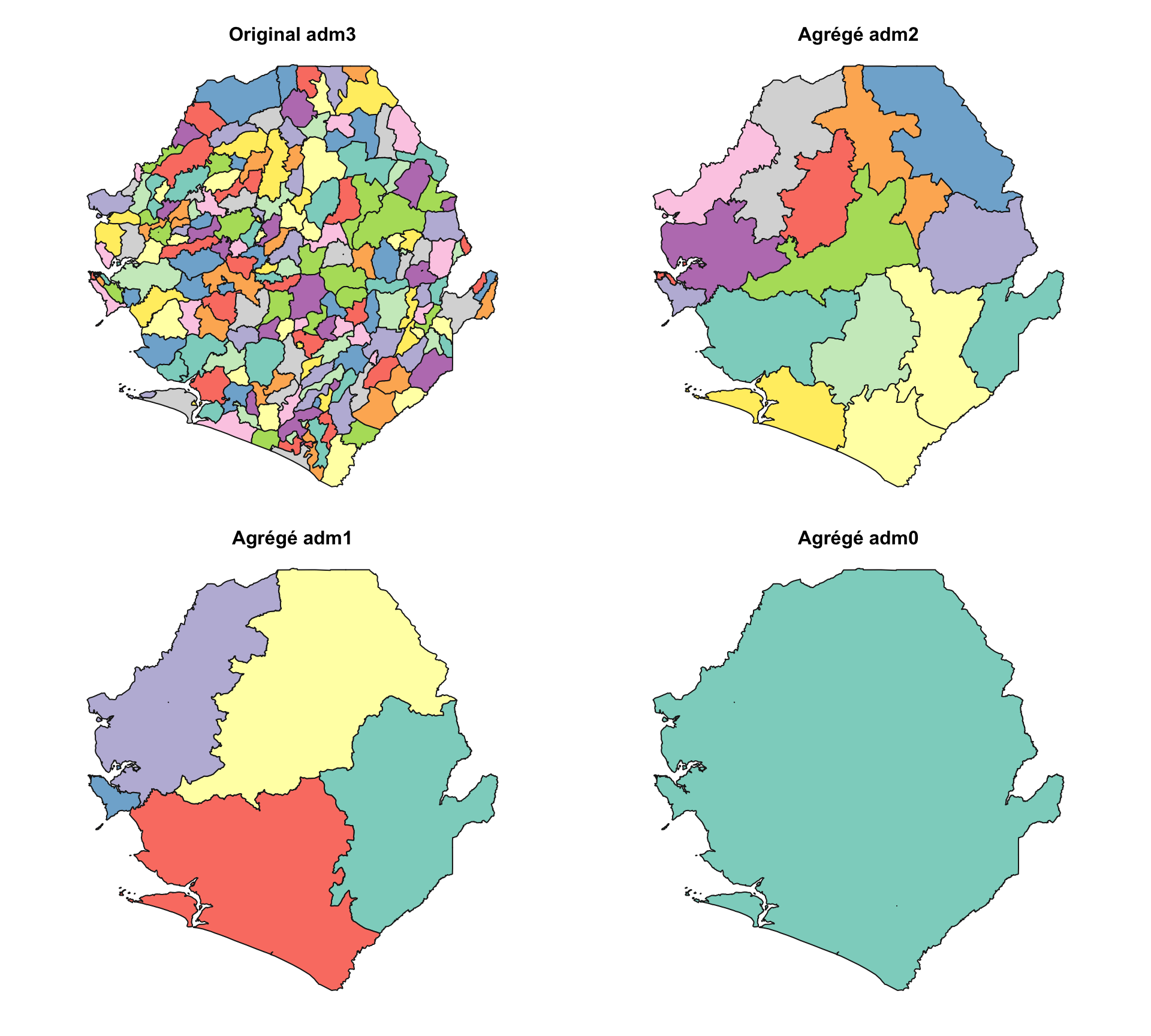
Étape 4 : Agréger ou reconstruire les limites administratives de niveau supérieur
Dans certains cas, les shapefiles peuvent n’être disponibles qu’à un niveau administratif inférieur (par exemple, adm3). Nous pouvons agréger ces unités adm3 pour construire des limites adm2, adm1 ou adm0.
Afficher le code
# créer un shapefile de niveau adm0 en
# regroupant sur le nom du pays
shp_adm0 <- shp_adm3 |>
dplyr::group_by(adm0) |>
dplyr::summarise(.groups = "drop") |>
sf::st_union(by_feature = TRUE)
# créer un shapefile de niveau adm1 en
# regroupant sur la région (par exemple, province)
shp_adm1 <- shp_adm3 |>
dplyr::group_by(adm0, adm1) |>
dplyr::summarise(.groups = "drop") |>
sf::st_union(by_feature = TRUE)
# créer un shapefile de niveau adm2 (par exemple, districts)
shp_adm2 <- shp_adm3 |>
dplyr::group_by(adm0, adm1, adm2) |>
dplyr::summarise(.groups = "drop") |>
sf::st_union(by_feature = TRUE)
# vérifier que les opérations ont fonctionné
# configurer une zone de tracé 2x2
graphics::par(mfrow = c(2, 2))
# définir les couleurs
plot_col <- sf::sf.colors(208, categorical = TRUE)
# tracer chaque niveau administratif
plot(shp_adm3$geometry, col = plot_col, main = "Original adm3")
plot(shp_adm2$geometry, col = plot_col, main = "Agrégé adm2 (de adm3)")
plot(shp_adm1$geometry, col = plot_col, main = "Agrégé adm1 (de adm3)")
plot(shp_adm0$geometry, col = plot_col, main = "Agrégé adm0 (de adm3)")
# réinitialiser la disposition de tracé (optionnel)
graphics::par(mfrow = c(1, 1))
NoteSortie
Pour adapter le code :
- Lignes 3, 10 et 16 : remplacez
shp_adm3par l’objet shapefile pertinent. - Lignes 4, 11–12 et 17–18 : mettez à jour les noms de colonnes (
adm0,adm1,adm2) pour correspondre à ceux de vos données. - Lignes 4, 11–12 et 17–18 : ajustez le niveau de regroupement en fonction du niveau administratif supérieur à créer.
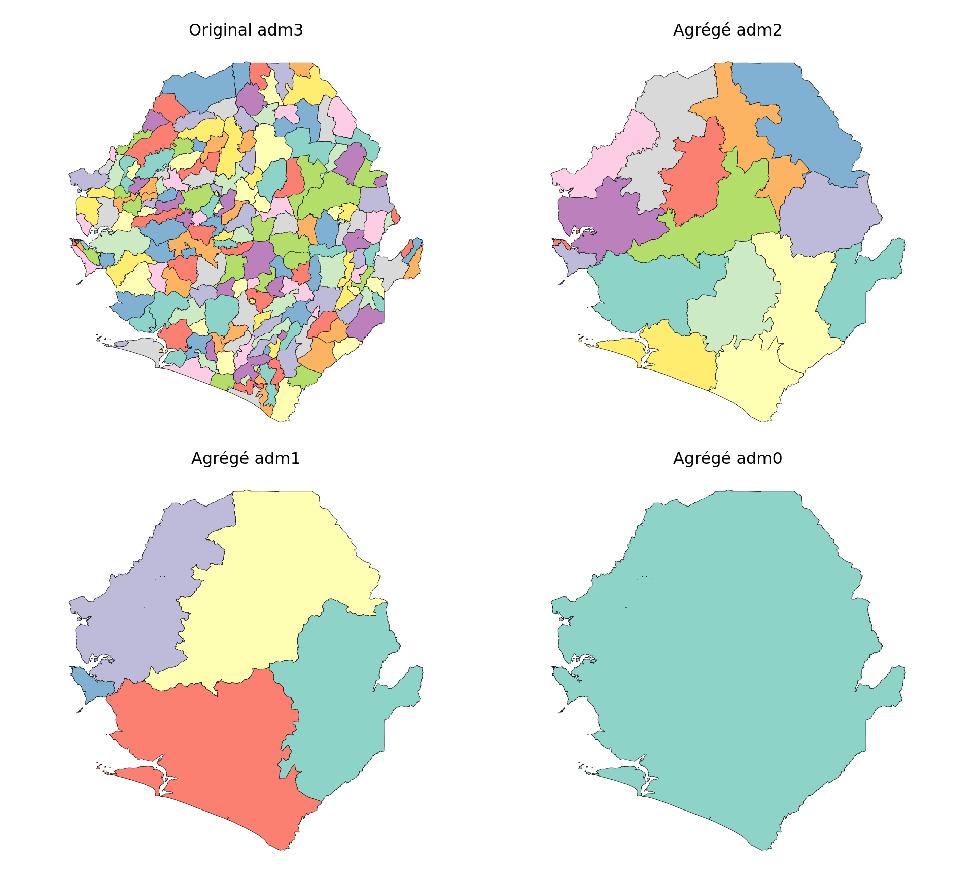
Afficher le code
# créer un shapefile de niveau adm0 en
# regroupant sur le nom du pays
shp_adm0 = shp_adm3[["adm0", "geometry"]].dissolve(
by="adm0",
as_index=False
)
# créer un shapefile de niveau adm1 en
# regroupant sur la région (par exemple, province)
shp_adm1 = shp_adm3[["adm0", "adm1", "geometry"]].dissolve(
by=["adm0", "adm1"],
as_index=False
)
# créer un shapefile de niveau adm2 (par exemple, districts)
shp_adm2 = shp_adm3[["adm0", "adm1", "adm2", "geometry"]].dissolve(
by=["adm0", "adm1", "adm2"],
as_index=False
)
# vérifier que les opérations ont fonctionné
# configurer une zone de tracé 2x2
fig, axes = plt.subplots(2, 2, figsize=(10, 9))
plt.subplots_adjust(
left=0.01,
right=0.99,
bottom=0.01,
top=0.95,
wspace=0.02,
hspace=0.08
)
# définir les couleurs
plot_col = sf_colors(208)
# tracer chaque niveau administratif
plot_sf_like(shp_adm3, ax=axes[0, 0], colors=plot_col, border="grey10",
title="Original adm3")
plot_sf_like(shp_adm2, ax=axes[0, 1], colors=plot_col, border="grey10",
title="Agrégé adm2")
plot_sf_like(shp_adm1, ax=axes[1, 0], colors=plot_col, border="grey10",
title="Agrégé adm1")
plot_sf_like(shp_adm0, ax=axes[1, 1], colors=plot_col, border="grey10",
title="Agrégé adm0")
plt.show()
NoteSortie
Pour adapter le code :
- Lignes 3, 10 et 17 : remplacez
shp_adm3par l’objet shapefile pertinent. - Lignes 3, 10–11 et 17–18 : mettez à jour les noms de colonnes (
adm0,adm1,adm2) pour correspondre à ceux de vos données. - Ajustez les colonnes de regroupement selon le niveau administratif supérieur à créer.
- Conservez
sf_colors(...)si vous voulez que les couleurs des graphiques Python correspondent à la sortiesf::sf.colors(..., categorical = TRUE)dans R.
Les tracés confirment que l’agrégation aux niveaux adm0, adm1 et adm2 a fonctionné comme prévu. Chaque carte montre des limites progressivement plus grossières, et la structure adm3 d’origine est préservée.
Étape 5 : Personnalisation des shapefiles
Étape 5.1 : Shapefiles de niveau mixte
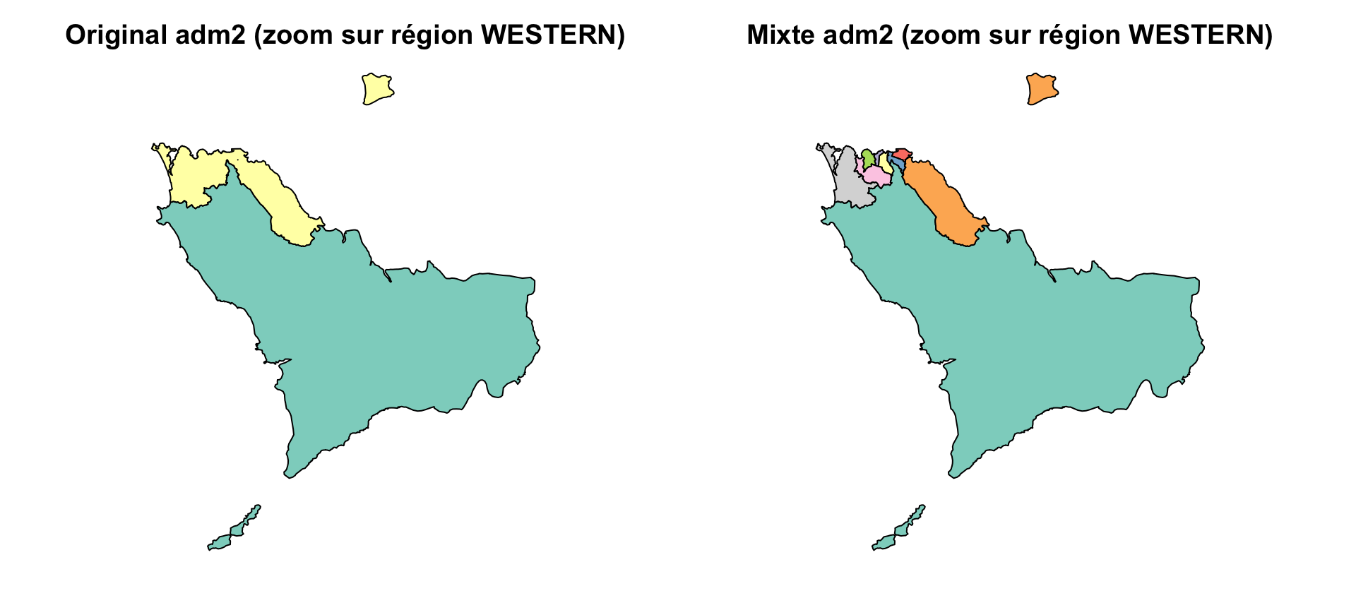
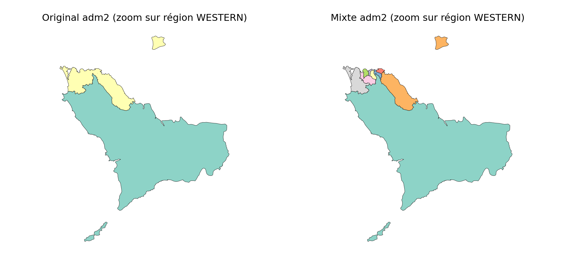
Dans certains cas, nous pouvons vouloir combiner différents niveaux administratifs au sein d’un même shapefile, par exemple, utiliser adm2 pour la plupart du pays tout en substituant des limites adm3 plus fines dans des zones sélectionnées. Cette approche est utile lorsque certains districts nécessitent plus de granularité pour l’analyse, la planification ou la visualisation, mais qu’un basculement complet vers adm3 n’est pas nécessaire.
Un cas d’utilisation pour cette approche est lorsque des détails géographiques plus fins ne sont nécessaires que dans des parties spécifiques du pays. Par exemple, en Sierra Leone, nous pouvons vouloir utiliser des limites adm3 dans Western Area Urban, qui comprend Freetown, une zone densément peuplée, tout en conservant des limites adm2 pour le reste du pays. Cela nous permet de maintenir une couverture nationale à une résolution gérable, tout en zoomant là où plus de granularité est nécessaire.
Afficher le code
# supprimer l'unité adm2 cible du shapefile adm2
target_adm2 <- "WESTERN URBAN"
adm2_trimmed <- shp_adm2 |>
dplyr::filter(adm2 != target_adm2)
# obtenir les unités adm3 équivalentes
adm3_subset <- shp_adm3 |>
dplyr::filter(adm2 == target_adm2)
# optionnel : ajouter une colonne pour indiquer le niveau source
adm2_trimmed <- adm2_trimmed |> dplyr::mutate(source = "adm2")
adm3_subset <- adm3_subset |> dplyr::mutate(source = "adm3")
# les combiner en un seul shapefile
shp_mixed <- dplyr::bind_rows(adm2_trimmed, adm3_subset)
# vérifier que les opérations ont fonctionné
# configurer une zone de tracé 1x2
graphics::par(mfrow = c(1, 2))
# définir les couleurs
plot_col <- sf::sf.colors(208, categorical = TRUE)
# tracer WESTERN pour montrer les changements plus fins
shp_adm2 |>
dplyr::filter(adm1 == "WESTERN") |>
sf::st_geometry() |>
plot(col = plot_col, main = "Original adm2 (zoom sur région WESTERN)")
shp_mixed |>
dplyr::filter(adm1 == "WESTERN") |>
sf::st_geometry() |>
plot(col = plot_col, main = "Mixte adm2 (zoom sur région WESTERN)")
# réinitialiser la disposition de tracé (optionnel)
graphics::par(mfrow = c(1, 1))
NoteSortie
Pour adapter le code :
Pour appliquer cela dans un autre contexte :
- Ligne 2 : remplacez
WESTERN URBANpar le nom de l’unité administrative à échanger. - Lignes 4–5, 8–9 : mettez à jour les noms de colonnes
adm2etadm3si le shapefile utilise des étiquettes différentes. - Répétez tout le bloc de code au besoin pour toutes les zones d’intérêt.
Afficher le code
# supprimer l'unité adm2 cible du shapefile adm2
target_adm2 = "WESTERN URBAN"
adm2_trimmed = shp_adm2.loc[shp_adm2["adm2"] != target_adm2].copy()
# obtenir les unités adm3 équivalentes
adm3_subset = shp_adm3.loc[shp_adm3["adm2"] == target_adm2].copy()
# optionnel : ajouter une colonne pour indiquer le niveau source
adm2_trimmed["source"] = "adm2"
adm3_subset["source"] = "adm3"
# les combiner en un seul shapefile
shp_mixed = gpd.GeoDataFrame(
pd.concat([adm2_trimmed, adm3_subset], ignore_index=True, sort=False),
geometry="geometry",
crs=shp_adm2.crs
)
# vérifier que les opérations ont fonctionné
# configurer une zone de tracé 1x2
fig, axes = plt.subplots(1, 2, figsize=(10, 4.5))
plt.subplots_adjust(
left=0.01,
right=0.99,
bottom=0.02,
top=0.90,
wspace=0.02
)
# définir les couleurs
plot_col = sf_colors(208)
# tracer WESTERN pour montrer les changements plus fins
plot_sf_like(
shp_adm2.loc[shp_adm2["adm1"] == "WESTERN"],
ax=axes[0],
colors=plot_col,
title="Original adm2 (zoom sur région WESTERN)"
)
plot_sf_like(
shp_mixed.loc[shp_mixed["adm1"] == "WESTERN"],
ax=axes[1],
colors=plot_col,
title="Mixte adm2 (zoom sur région WESTERN)"
)
plt.show()
NoteSortie
Pour adapter le code :
- Ligne 2 : remplacez
WESTERN URBANpar le nom de l’unité administrative à échanger. - Lignes 4–5 et 8–9 : mettez à jour les noms de colonnes
adm2etadm3si le shapefile utilise des étiquettes différentes. - Lignes 12–13 : mettez à jour les valeurs
sourcesi vous voulez utiliser d’autres étiquettes pour la couche de niveau mixte. - Répétez le même modèle pour chaque zone où un niveau administratif doit être remplacé par un niveau plus fin.
Les résultats montrent que l’opération a fonctionné : dans la région WESTERN, Western Rural reste une unité adm2 unique, tandis que Western Urban a été remplacé avec succès par plusieurs unités adm3 plus fines. Cette vue zoomée montre des différences non visibles à l’échelle nationale. Bien que shp_mixed inclue toutes les régions, cette comparaison confirme la substitution ciblée.
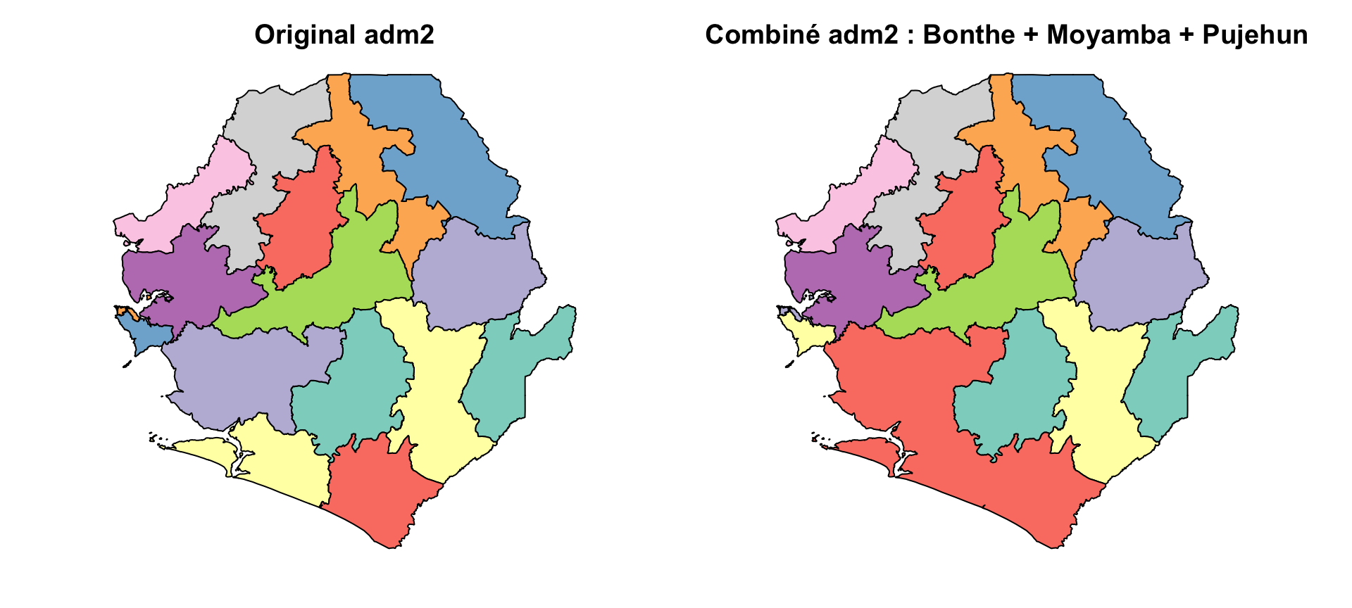
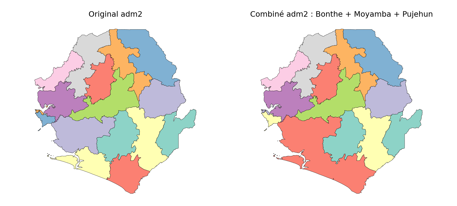
Étape 5.2 : Fusion de plusieurs polygones en une seule unité
Dans certains cas, il peut être nécessaire de fusionner deux ou plusieurs unités administratives adjacentes en une seule entité géographique. Cela pourrait être fait pour la commodité opérationnelle, la simplicité de reporting ou lorsque de petites unités voisines doivent être traitées comme une seule zone de planification.
Par exemple, nous montrons comment trois districts du sud de la Sierra Leone (Bonthe, Moyamba et Pujehun) peuvent être combinés en une seule unité.
Afficher le code
# définir les unités adm2 à combiner
combine_names <- c("BONTHE", "MOYAMBA", "PUJEHUN")
# créer une nouvelle unité combinée
combined <- shp_adm2 |>
dplyr::filter(adm2 %in% combine_names) |>
dplyr::summarise(
adm3 = paste(combine_names, collapse = " ~ "),
geometry = sf::st_union(geometry),
.groups = "drop"
)
# supprimer les originaux et lier la nouvelle unité
shp_adm2_combined <- shp_adm2 |>
dplyr::filter(!adm2 %in% combine_names) |>
dplyr::bind_rows(combined)
# vérifier que les opérations ont fonctionné
# configurer une zone de tracé 1x2
graphics::par(mfrow = c(1, 2))
# définir les couleurs
plot_col <- sf::sf.colors(10, categorical = TRUE)
# tracer chaque niveau administratif
plot(shp_adm2$geometry, col = plot_col, main = "Original adm2")
plot(
shp_adm2_combined$geometry,
col = plot_col,
main = "Combiné adm2 : Bonthe + Moyamba + Pujehun"
)
# réinitialiser la disposition de tracé (optionnel)
graphics::par(mfrow = c(1, 1))
NoteSortie
Pour adapter le code :
- Ligne 2 : changez les noms dans
combine_namespour les unités à fusionner. - Lignes 6, 15 : mettez à jour le champ adm2 si le shapefile utilise un nom différent (par exemple,
district_name). - Ligne 8 : ajustez le nom de sortie (
adm3 = paste(...)) pour refléter comment l’unité fusionnée doit être étiquetée, par exemple, utilisezSouthern Clusterà la place. - Répétez tout le bloc de code au besoin pour toutes les zones d’intérêt.
Afficher le code
# définir les unités adm2 à combiner
combine_names = ["BONTHE", "MOYAMBA", "PUJEHUN"]
# créer une nouvelle unité combinée
combined = gpd.GeoDataFrame(
{
"adm3": [" ~ ".join(combine_names)],
"geometry": [
unary_union(
shp_adm2.loc[shp_adm2["adm2"].isin(combine_names), "geometry"]
)
],
},
geometry="geometry",
crs=shp_adm2.crs
)
# supprimer les originaux et lier la nouvelle unité
shp_adm2_combined = gpd.GeoDataFrame(
pd.concat(
[
shp_adm2.loc[~shp_adm2["adm2"].isin(combine_names)],
combined,
],
ignore_index=True,
sort=False
),
geometry="geometry",
crs=shp_adm2.crs
)
# vérifier que les opérations ont fonctionné
# configurer une zone de tracé 1x2
fig, axes = plt.subplots(1, 2, figsize=(10, 4.5))
plt.subplots_adjust(
left=0.01,
right=0.99,
bottom=0.02,
top=0.90,
wspace=0.02
)
# définir les couleurs
plot_col = sf_colors(10)
# tracer chaque niveau administratif
plot_sf_like(shp_adm2, ax=axes[0], colors=plot_col, title="Original adm2")
plot_sf_like(
shp_adm2_combined,
ax=axes[1],
colors=plot_col,
title="Combiné adm2 : Bonthe + Moyamba + Pujehun"
)
plt.show()
NoteSortie
Pour adapter le code :
- Ligne 2 : changez les noms dans
combine_namespour les unités à fusionner. - Lignes 9 et 25 : mettez à jour le champ
adm2si le shapefile utilise un nom différent, par exempledistrict_name. - Ligne 7 : ajustez le nom de sortie (
" ~ ".join(combine_names)) pour refléter comment l’unité fusionnée doit être étiquetée. - Répétez le même bloc de code au besoin pour toutes les unités fusionnées personnalisées.
Le tracé montre que les districts sélectionnés ont été fusionnés avec succès en un seul polygone, formant une unité géographique personnalisée.
Étape 6 : Créer des ID géographiques et comparer les versions
Pour suivre les changements dans la géométrie des limites au fil du temps ou entre les versions de shapefile, nous générons un ID d’empreinte basé sur la géométrie pour chaque polygone. Cela nous permet de détecter si une unité a changé spatialement, même si son nom reste le même. Nous utilisons ensuite ces empreintes pour comparer deux versions du même shapefile et visualiser ce qui a changé.
Étape 6.1 : Créer des empreintes de géométrie
Cette étape est utile pour vérifier les mises à jour de shapefile, aligner les géographies entre les années et s’assurer que les comparaisons historiques sont faites correctement. Nous pouvons également utiliser des empreintes de géométrie pour vérifier les polygones en double dans le même shapefile (étape 3 ci-dessus).
Afficher le code
# créer un ID d'empreinte pour chaque polygone en utilisant sa géométrie
shp_adm3 <- shp_adm3 |>
dplyr::mutate(
geometry_hash = sntutils::vdigest(geometry, algo = "xxhash32")
) |>
dplyr::select(adm0, adm1, adm2, adm3, geometry_hash)
shp_adm2 <- shp_adm2 |>
dplyr::mutate(
geometry_hash = sntutils::vdigest(geometry, algo = "xxhash32")
) |>
dplyr::select(adm0, adm1, adm2, geometry_hash)
shp_adm1 <- shp_adm1 |>
dplyr::mutate(
geometry_hash = sntutils::vdigest(geometry, algo = "xxhash32")
) |>
dplyr::select(adm0, adm1, geometry_hash)
shp_adm0 <- shp_adm0 |>
dplyr::mutate(
geometry_hash = sntutils::vdigest(geometry, algo = "xxhash32")
) |>
dplyr::select(adm0, geometry_hash)
# vérifier l'unicité de chaque ID d'empreinte de forme
cli::cli_h2("Vérification de l'unicité des ID d'empreinte")
adm0_n <- nrow(shp_adm0)
adm0_unique <- dplyr::n_distinct(shp_adm0$geometry_hash)
cli::cli_alert_info("adm0 : {adm0_unique} empreintes uniques sur {adm0_n} lignes")
adm1_n <- nrow(shp_adm1)
adm1_unique <- dplyr::n_distinct(shp_adm1$geometry_hash)
cli::cli_alert_info("adm1 : {adm1_unique} empreintes uniques sur {adm1_n} lignes")
adm2_n <- nrow(shp_adm2)
adm2_unique <- dplyr::n_distinct(shp_adm2$geometry_hash)
cli::cli_alert_info("adm2 : {adm2_unique} empreintes uniques sur {adm2_n} lignes")
adm3_n <- nrow(shp_adm3)
adm3_unique <- dplyr::n_distinct(shp_adm3$geometry_hash)
cli::cli_alert_info("adm3 : {adm3_unique} empreintes uniques sur {adm3_n} lignes")
# vérifier la sortie
head(shp_adm3)Pour adapter le code :
- Lignes 2, 8, 14 et 20 : remplacez
shp_adm3,shp_adm2, etc. par les objets shapefile pertinents. - Assurez-vous que chaque couche a une colonne de géométrie de classe
sfc. - Lignes 6, 12, 18 et 24 : les noms de champs (
adm0,adm1, etc.) peuvent être ajustés pour correspondre au schéma de nommage en usage.
Afficher le code
# créer un ID d'empreinte pour chaque polygone en utilisant sa géométrie
shp_adm3 = (
shp_adm3.assign(
geometry_hash=shp_adm3.geometry.apply(lambda x: geometry_hash(x, "xxhash32"))
)
[["adm0", "adm1", "adm2", "adm3", "geometry_hash", "geometry"]]
)
shp_adm2 = (
shp_adm2.assign(
geometry_hash=shp_adm2.geometry.apply(lambda x: geometry_hash(x, "xxhash32"))
)
[["adm0", "adm1", "adm2", "geometry_hash", "geometry"]]
)
shp_adm1 = (
shp_adm1.assign(
geometry_hash=shp_adm1.geometry.apply(lambda x: geometry_hash(x, "xxhash32"))
)
[["adm0", "adm1", "geometry_hash", "geometry"]]
)
shp_adm0 = (
shp_adm0.assign(
geometry_hash=shp_adm0.geometry.apply(lambda x: geometry_hash(x, "xxhash32"))
)
[["adm0", "geometry_hash", "geometry"]]
)
# vérifier l'unicité de chaque ID d'empreinte de forme
cli_header("Vérification de l'unicité des ID d'empreinte")
adm0_n = len(shp_adm0)
adm0_unique = shp_adm0["geometry_hash"].nunique()
cli_info(f"adm0 : {adm0_unique} empreintes uniques sur {adm0_n} lignes")
adm1_n = len(shp_adm1)
adm1_unique = shp_adm1["geometry_hash"].nunique()
cli_info(f"adm1 : {adm1_unique} empreintes uniques sur {adm1_n} lignes")
adm2_n = len(shp_adm2)
adm2_unique = shp_adm2["geometry_hash"].nunique()
cli_info(f"adm2 : {adm2_unique} empreintes uniques sur {adm2_n} lignes")
adm3_n = len(shp_adm3)
adm3_unique = shp_adm3["geometry_hash"].nunique()
cli_info(f"adm3 : {adm3_unique} empreintes uniques sur {adm3_n} lignes")
# vérifier la sortie
shp_adm3.head()Pour adapter le code :
- Lignes 2, 9, 16 et 23 : remplacez
shp_adm3,shp_adm2, etc. par les objets shapefile pertinents. - Assurez-vous que chaque couche a une colonne
geometryvalide. - Lignes 6, 13, 20 et 27 : ajustez les noms de champs sélectionnés (
adm0,adm1, etc.) pour correspondre au schéma de nommage en usage. - Conservez le même algorithme de hachage pour toutes les couches et toutes les versions de shapefile à comparer.
Nous avons maintenant des shapefiles propres pour chaque niveau administratif (adm0–adm3), chacun étiqueté avec un ID d’empreinte basé sur la géométrie.
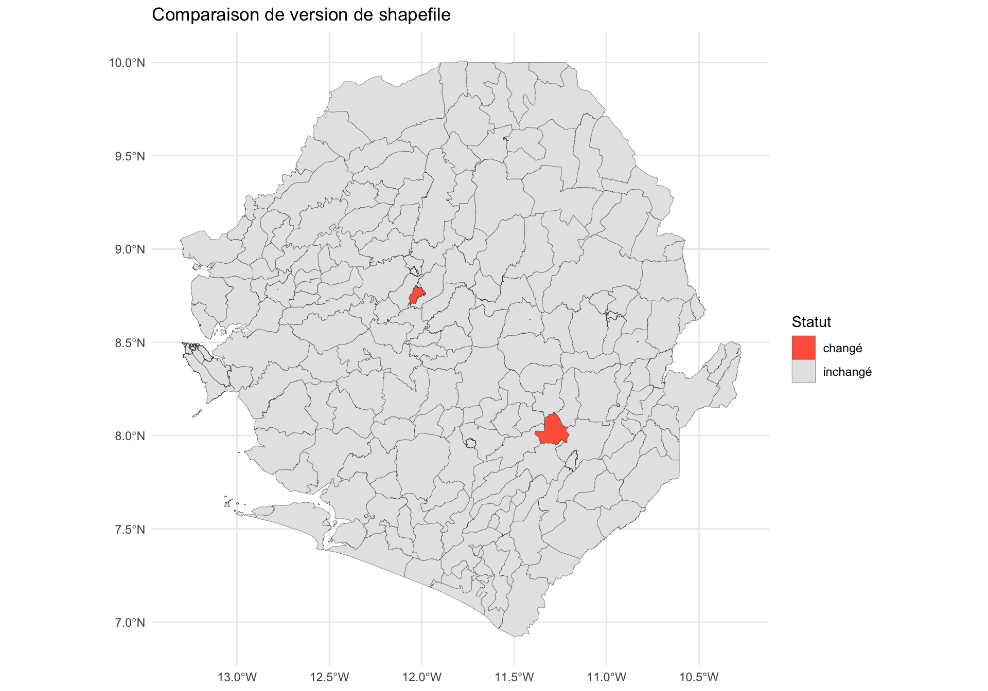
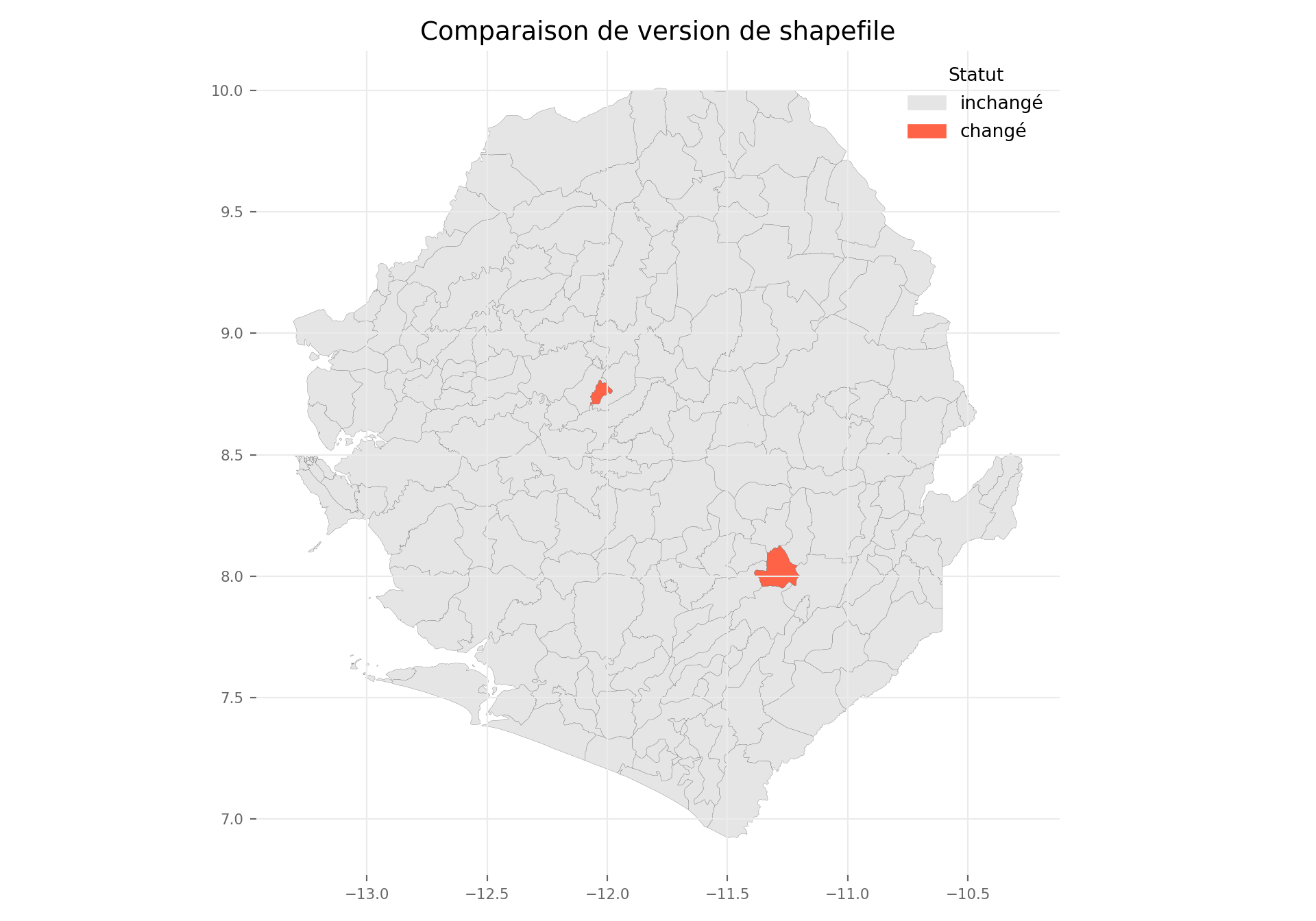
Étape 6.2 : Comparer deux versions de shapefile visuellement
Une fois que chaque polygone a une empreinte de géométrie, nous pouvons comparer une version précédente du shapefile par rapport à la version actuelle pour voir exactement quelles unités ont changé. Nous joignons les deux versions par leurs clés de nom d’administration, classons chaque unité comme inchangé, changé, nouveau ou supprimé, et superposons le résultat sur une carte.
Pour cette démo, nous simulons une « version précédente » (shp_adm3_v0) en perturbant quelques polygones du shp_adm3 actuel. En usage réel, shp_adm3_v0 serait chargé à partir d’un shapefile plus ancien stocké séparément.
Afficher le code
# charger la version précédente (ici nous la simulons à partir de shp_adm3)
shp_adm3_v0 <- shp_adm3 |>
# perturber la géométrie de deux chefferies pour simuler des redessins de limites
dplyr::mutate(
geometry = ifelse(
seq_len(dplyr::n()) %in% c(20, 50),
sf::st_buffer(geometry, dist = 0.01),
geometry
)
) |>
sf::st_as_sf() |>
dplyr::mutate(
geometry_hash = sntutils::vdigest(geometry, algo = "xxhash32")
)
# joindre les deux versions sur les clés de nom d'administration et comparer les empreintes
join_keys <- c("adm0", "adm1", "adm2", "adm3")
diff_df <- shp_adm3 |>
sf::st_drop_geometry() |>
dplyr::full_join(
shp_adm3_v0 |> sf::st_drop_geometry(),
by = join_keys,
suffix = c("_new", "_old")
) |>
dplyr::mutate(
status = dplyr::case_when(
is.na(geometry_hash_old) ~ "nouveau",
is.na(geometry_hash_new) ~ "supprimé",
geometry_hash_new != geometry_hash_old ~ "changé",
TRUE ~ "inchangé"
)
)
# rattacher le statut à la version actuelle et tracer
shp_adm3_diff <- shp_adm3 |>
dplyr::left_join(
diff_df |> dplyr::select(dplyr::all_of(join_keys), status),
by = join_keys
)
ggplot2::ggplot(shp_adm3_diff) +
ggplot2::geom_sf(ggplot2::aes(fill = status), colour = "grey30", size = 0.1) +
ggplot2::scale_fill_manual(values = c(
inchangé = "grey90",
changé = "tomato",
nouveau = "skyblue",
supprimé = "orange"
)) +
ggplot2::labs(
title = "Comparaison de version de shapefile",
fill = "Statut"
) +
ggplot2::theme_minimal()
NoteSortie
Pour adapter le code :
- Ligne 2 : remplacez le
shp_adm3_v0simulé par le shapefile précédent réel, chargé viasf::read_sf()et traité à travers les étapes 2–6.1 pour attacher des empreintes de géométrie. - Ligne 16 : mettez à jour
join_keyspour correspondre aux colonnes de nom d’administration dans les données. - Lignes 40–47 : ajustez la palette de couleurs et les étiquettes pour correspondre au style de rapport.
- Le même modèle fonctionne pour les niveaux administratifs supérieurs en substituant
shp_adm2,shp_adm1, etc.
Afficher le code
# charger la version précédente (ici nous la simulons à partir de shp_adm3)
shp_adm3_v0 = shp_adm3.copy()
# perturber la géométrie de deux chefferies pour simuler des redessins de limites
rows_to_change = shp_adm3_v0.index[[19, 49]]
shp_adm3_v0.loc[rows_to_change, "geometry"] = (
shp_adm3_v0.loc[rows_to_change, "geometry"].buffer(0.01)
)
shp_adm3_v0 = shp_adm3_v0.assign(
geometry_hash=shp_adm3_v0.geometry.apply(lambda x: geometry_hash(x, "xxhash32"))
)
# joindre les deux versions sur les clés de nom d'administration et comparer les empreintes
join_keys = ["adm0", "adm1", "adm2", "adm3"]
diff_df = (
shp_adm3.drop(columns="geometry")
.merge(
shp_adm3_v0.drop(columns="geometry"),
on=join_keys,
how="outer",
suffixes=("_new", "_old")
)
)
diff_df["status"] = np.select(
[
diff_df["geometry_hash_old"].isna(),
diff_df["geometry_hash_new"].isna(),
diff_df["geometry_hash_new"] != diff_df["geometry_hash_old"],
],
["nouveau", "supprimé", "changé"],
default="inchangé"
)
# rattacher le statut à la version actuelle et tracer
shp_adm3_diff = shp_adm3.merge(
diff_df[join_keys + ["status"]],
on=join_keys,
how="left"
)
status_colors = {
"inchangé": "grey90",
"changé": "tomato",
"nouveau": "skyblue",
"supprimé": "orange",
}
fig, ax = plt.subplots(figsize=(10, 7))
for status, color in status_colors.items():
subset = shp_adm3_diff.loc[shp_adm3_diff["status"] == status]
if not subset.empty:
subset.plot(
ax=ax,
color=r_color(color),
edgecolor=r_color("grey30"),
linewidth=0.1,
)
legend_handles = [
mpatches.Patch(color=r_color(color), label=status)
for status, color in status_colors.items()
if status in set(shp_adm3_diff["status"].dropna())
]
ax.legend(handles=legend_handles, title="Statut", frameon=False)
ax.set_title("Comparaison de version de shapefile", fontsize=14)
ax.grid(True, color="#ebebeb", linewidth=0.8)
ax.tick_params(labelsize=8, colors="#666666")
for spine in ax.spines.values():
spine.set_visible(False)
plt.tight_layout()
plt.show()
NoteSortie
Pour adapter le code :
- Ligne 2 : remplacez le
shp_adm3_v0simulé par le shapefile précédent réel, chargé avecgpd.read_file()et traité à travers les étapes 2–6.1 pour attacher des empreintes de géométrie. - Ligne 14 : mettez à jour
join_keyspour correspondre aux colonnes de nom d’administration dans les données. - Lignes 39–44 : ajustez la palette de couleurs et les étiquettes pour correspondre au style de rapport.
- Le même modèle fonctionne pour les niveaux administratifs supérieurs en substituant
shp_adm2,shp_adm1, etc.
La carte met en évidence les deux chefferies perturbées en rouge (changé), le reste du pays étant affiché comme inchangé. Dans une comparaison réelle, les unités nouveau apparaîtraient là où le shapefile plus récent a ajouté un polygone (par exemple, une division de district) et les unités supprimé là où un polygone a été retiré. Ce diff visuel est plus rapide que l’examen des tables d’attributs ligne par ligne et permet de signaler facilement les zones affectées à l’équipe SNT.
Étape 7 : Enregistrement des données vectorielles
Après avoir nettoyé et transformé les données spatiales, il est important de les enregistrer dans un format qui préserve la géométrie, la structure et le CRS. R prend en charge plusieurs formats vectoriels, et nous n’avons pas besoin de tous les utiliser ; choisissez simplement les formats qui correspondent au flux de travail et à la manière dont les données seront réutilisées ou partagées.
Voici les principales options, avec des notes sur quand et comment les utiliser. Utilisez celle(s) qui fonctionne(nt) le mieux pour l’équipe et le contexte.
Afficher le code
# enregistrer adm0
saveRDS(
shp_adm0,
here::here(
spat_path, "processed", "sle_spatial_adm0_2021.rds"
)
)
# enregistrer adm1
saveRDS(
shp_adm1,
here::here(
spat_path, "processed", "sle_spatial_adm1_2021.rds"
)
)
# enregistrer adm2
saveRDS(
shp_adm2,
here::here(
spat_path, "processed", "sle_spatial_adm2_2021.rds"
)
)
# enregistrer adm3
saveRDS(
shp_adm3,
here::here(
spat_path, "processed", "sle_spatial_adm3_2021.rds"
)
)L’exemple ci-dessus montre comment enregistrer des shapefiles de plusieurs niveaux administratifs en utilisant à la fois les fonctions RDS et st_write. Choisissez le format qui correspond le mieux au flux de travail, que ce soit le stockage de couches ensemble ou leur exportation individuellement.
Si l’objet spatial a été enregistré en utilisant saveRDS(), nous pouvons le charger avec readRDS() et le convertir en un objet sf :
GeoJSON (.geojson) : pour les fichiers GeoJSON :
GeoPackage (.gpkg) : pour les fichiers GeoPackage :
File Geodatabase (.gdb) : pour les fichiers Geodatabase :
sf::st_write(
shp_adm3, # objet à écrire
here::here("folder", "boundary.gdb"), # chemin de la géodatabase de sortie
layer = "adm3", # nom de la couche à l'intérieur de gdb
driver = "FileGDB", # utiliser le pilote FileGDB
delete_layer = TRUE, # écraser la couche si elle existe
quiet = TRUE # masquer les messages d'écriture
)Pour adapter le code :
- Lignes 2–4, 7–10, 13–16 et 19–22 : adaptez les chemins de fichiers et les noms de colonnes (
adm0,adm1,adm2,adm3) en fonction de la structure de dossiers pertinente et des données spécifiques au pays. Tous les pays n’utilisent pas de niveauadm3, donc cela variera en fonction du contexte. - Choisissez le format qui correspond le mieux au flux de travail :
RDSpour une réutilisation native dans R,GeoJSONpour une large compatibilité,GeoPackagepour les fichiers spatiaux multi-couches, ou File Geodatabase pour les pipelines ArcGIS. - Utilisez
readRDS()suivi desf::st_as_sf()pour charger un objet spatial préalablement enregistré avecsaveRDS().
Python n’écrit pas directement des fichiers .rds natifs de R. Pour un flux de travail Python, utilisez des formats spatiaux ouverts comme GeoJSON ou GeoPackage, ou GeoParquet pour une réutilisation efficace dans Python. Si le flux de travail en aval exige spécifiquement un fichier .rds, créez cette copie depuis R.
Afficher le code
processed_path = Path(spat_path) / "processed"
processed_path.mkdir(parents=True, exist_ok=True)
# enregistrer adm0
shp_adm0.to_file(
processed_path / "sle_spatial_adm0_2021.geojson",
driver="GeoJSON"
)
# enregistrer adm1
shp_adm1.to_file(
processed_path / "sle_spatial_adm1_2021.geojson",
driver="GeoJSON"
)
# enregistrer adm2
shp_adm2.to_file(
processed_path / "sle_spatial_adm2_2021.geojson",
driver="GeoJSON"
)
# enregistrer adm3
shp_adm3.to_file(
processed_path / "sle_spatial_adm3_2021.geojson",
driver="GeoJSON"
)GeoJSON (.geojson) : pour les fichiers GeoJSON :
GeoPackage (.gpkg) : pour les fichiers GeoPackage :
GeoParquet (.parquet) : pour les flux de travail Python efficaces :
File Geodatabase (.gdb) : pour les fichiers Geodatabase, la prise en charge du pilote dépend de l’installation GDAL locale :
Pour adapter le code :
- Lignes 1–2 : mettez à jour
processed_pathpour correspondre à la structure de dossiers de votre projet. - Lignes 5, 11, 17 et 23 : remplacez les noms d’objets (
shp_adm0,shp_adm1, etc.) si votre flux de travail utilise des noms différents. - Mettez à jour les noms de fichiers de sortie pour correspondre au code pays, au niveau administratif et à l’année des limites.
- Utilisez GeoJSON pour une large compatibilité, GeoPackage pour des fichiers spatiaux multi-couches, ou GeoParquet pour les flux de travail Python efficaces.
- Si une autre partie du flux de travail SNT exige un
.rds, créez ce fichier depuis l’onglet R plutôt que depuis Python.
TipListe de contrôle qualité du shapefile SNT
Avant de passer à toute analyse en aval, confirmez que le shapefile nettoyé passe toutes les vérifications suivantes. Si l’une échoue, retournez à l’étape pertinente ci-dessus.
- Géométries valides :
sf::st_is_valid()dans R, ou.geometry.is_validdans Python, retourneTRUE/Truepour chaque entité (étape 3.1). - Polygones uniques : aucun doublon de ligne complète ou de géométrie uniquement ne reste, en utilisant
dplyr::distinct()/sf::st_as_binary()dans R ou.drop_duplicates()/les vérifications WKB dans Python (étapes 3.2–3.3). - CRS cohérent : chaque couche utilise le même CRS, généralement
EPSG:4326, vérifié avecsf::st_crs()dans R ou.crsdans Python (étape 2.2). - Aucune erreur de topologie : aucun trou interne ou fine bande adjacente détecté dans le résumé de topologie R ou Python (étape 3.4).
- Hiérarchie administrative alignée : les couches
adm0,adm1,adm2(etadm3) s’emboîtent proprement lorsqu’elles sont agrégées avecdplyr::summarise()/sf::st_union()dans R ou.dissolve()dans Python (étape 4). - ID d’empreinte de géométrie : une colonne
geometry_hashunique est attachée à chaque niveau administratif avecsntutils::vdigest()dans R ou la fonction d’aide Pythongeometry_hash()(étape 6.1). - Version suivie : lorsqu’un shapefile mis à jour arrive, le diff par rapport à la version précédente a été examiné dans R ou Python (étape 6.2).
- Enregistré durablement : les couches nettoyées sont écrites dans des formats stables, tels que
.rds,.gpkgou.geojsondans R et.geojson,.gpkgou GeoParquet dans Python, avec un nommage de fichier cohérent (étape 7).
Conservez cette liste de contrôle à côté du shapefile pour chaque projet SNT afin que les mêmes normes s’appliquent à chaque pays et à chaque actualisation.
Résumé
Cette section fournit une base pratique pour gérer les données shapefile dans le flux de travail SNT. Elle parcourt les étapes clés nécessaires pour préparer, valider et personnaliser les couches de limites. Elle offre des solutions pour résoudre les problèmes de géométrie, gérer les doublons, aligner les CRS, détecter les trous topologiques et les fines bandes, et construire des couches administratives flexibles adaptées aux besoins du programme. La page introduit également le hachage de géométrie pour soutenir le suivi de version, démontre comment comparer et visualiser les différences entre deux versions de shapefile, et montre comment exporter des données spatiales nettoyées pour l’analyse et la cartographie. Ces étapes garantissent que toutes les opérations spatiales dans le SNT sont construites sur une base géographique stable et reproductible.
Les analystes peuvent revenir à des étapes spécifiques au besoin tout au long de leur travail, faisant de cette page une référence à long terme pour une préparation cohérente des données spatiales dans les projets SNT.
Code complet
Trouvez le script de code complet pour gérer et personnaliser les shapefiles ci-dessous.
Show full code
################################################################################
########### ~ Gestion et personnalisation des shapefiles full code ~ ###########
################################################################################
### Step -----------------------------------------------------------------------
# installer `pacman` s'il n'est pas déjà installé
if (!requireNamespace("pacman", quietly = TRUE)) {
install.packages("pacman")
}
# charger les paquets requis en utilisant pacman
pacman::p_load(
sf, # gestion des données shapefile
dplyr, # manipulation de données
ggplot2, # tracé
here, # gestion des chemins de fichiers
stringr, # manipulation de chaînes (par exemple, str_remove)
cli, # journalisation propre et messages de style CLI
devtools # pour la gestion des paquets
)
# sntutils a un certain nombre de fonctions d'aide utiles pour
# la gestion et le nettoyage des données
if (!requireNamespace("sntutils", quietly = TRUE)) {
devtools::install_github("ahadi-analytics/sntutils")
}
# configurer le chemin spatial
spat_path <- here::here(
"01_data", "1.1_foundational", "1.1a_admin_boundaries"
)
# importer le shapefile
shp_adm3 <- sf::read_sf(
here::here(spat_path, "raw", "Chiefdom2021.shp")
) |>
dplyr::mutate(adm0 = "SIERRA LEONE") |>
dplyr::select(
# sélectionner les colonnes pertinentes et renommer selon la nomenclature standard
adm0,
adm1 = FIRST_REGI,
adm2 = FIRST_DNAM,
adm3 = FIRST_CHIE
) |>
# garantir que la sortie reste un objet sf valide pour une utilisation en aval
sf::st_as_sf()
# vérifier la sortie par cartographie
plot(shp_adm3)
cli::cli_h2("Vérifier et attribuer la CRS d'origine pour shp_adm3")
shp_adm3 <- sf::st_set_crs(shp_adm3, 4326)
cli::cli_alert_info("CRS d'origine : {sf::st_crs(shp_adm3)$input}")
# transformer en nouvelle CRS (par exemple, Equal Earth - EPSG:6933)
shp_adm3_diff_crs <- sf::st_transform(shp_adm3, 6933)
cli::cli_h2("Vérifier la CRS après transformation")
cli::cli_alert_info("Nouvelle CRS : {sf::st_crs(shp_adm3_diff_crs)$input}")
# vérifier la validité de la géométrie
shp_adm3_inv <- shp_adm3 |>
dplyr::mutate(
valid = sf::st_is_valid(geometry),
invalid_reason = sf::st_is_valid(geometry, reason = TRUE),
invalid_reason = stringr::str_remove(invalid_reason, "\\[.*")
)
# obtenir la liste des adm3 invalides
invalid_df <- shp_adm3_inv |>
dplyr::filter(!valid) |>
sf::st_drop_geometry() |>
dplyr::select(adm0, adm1, adm2, adm3, invalid_reason)
# afficher les lignes invalides (le cas échéant)
invalid_df
# corriger les problèmes de géométrie connus
# (par exemple, auto-intersections, anneaux non fermés)
shp_adm3 <- shp_adm3 |>
sf::st_make_valid()
# revérifier et signaler les géométries invalides restantes
n_invalid <- shp_adm3 |>
dplyr::mutate(valid = sf::st_is_valid(geometry)) |>
dplyr::filter(!valid) |>
nrow()
cli::cli_alert_info("Géométries invalides restantes : {n_invalid}")
# vérifier les géométries en double
shp_adm3_dup <- shp_adm3 |>
  dplyr::mutate(dup_geom = duplicated(sf::st_as_binary(geometry))) |>
  dplyr::filter(dup_geom == TRUE)

cli::cli_alert_info("Nombre de géométries en double : {nrow(shp_adm3_dup)}")
# vérifier les doublons de ligne complète
dups_full <- shp_adm3 |>
dplyr::group_by(dplyr::across(dplyr::everything())) |>
dplyr::filter(dplyr::n() > 1)
# vérifier les doublons de géométrie uniquement
dups_geom <- shp_adm3 |>
dplyr::mutate(geom_hash = sntutils::vdigest(geometry)) |>
dplyr::add_count(geom_hash, name = "n_geom") |>
dplyr::filter(n_geom > 1)
# afficher les résultats
cli::cli_h1("Vérification des doublons de ligne complète")
dups_full |> sf::st_drop_geometry()
cli::cli_h1("Vérification des doublons de géométrie uniquement")
dups_geom |> sf::st_drop_geometry()
# supprimer les doublons de ligne complète
shp_adm3 <- shp_adm3 |>
dplyr::distinct()
# si nécessaire, supprimer les doublons de géométrie uniquement connus en filtrant sur les étiquettes
# supprimer l'étiquette intentionnellement dupliquée
shp_adm3 <- shp_adm3 |>
dplyr::filter(adm3 != "DUPLICATE LABEL")
# vérifier à nouveau après nettoyage
# vérifier les doublons de géométrie uniquement dans shp_adm3
shp_adm3_dup <- shp_adm3 |>
dplyr::mutate(dup_geom = duplicated(sf::st_as_binary(geometry))) |>
dplyr::filter(dup_geom == TRUE)
cli::cli_alert_info(
"Nombre de géométries en double dans shp_adm3 : {nrow(shp_adm3_dup)}"
)
# détecter les chevauchements adjacents (fines bandes) en intersectant la couche avec elle-même
overlaps <- shp_adm3 |>
sf::st_intersection() |>
dplyr::filter(n.overlaps > 1) |>
dplyr::mutate(
overlap_area_m2 = as.numeric(sf::st_area(geometry))
) |>
# supprimer les vraies intersections point/ligne (surface nulle) et le bruit numérique
dplyr::filter(overlap_area_m2 > 1)
cli::cli_alert_info(
"Entités de chevauchement adjacent détectées : {nrow(overlaps)}"
)
# détecter les trous internes en comptant les anneaux intérieurs dans l'union du pays.
# utiliser une union planaire (GEOS) pour que le comptage des trous corresponde à l'onglet
# python, qui unit aussi avec GEOS - l'union sphérique s2 accroche les petites fines
# bandes différemment et signale un nombre de trous différent
s2_was_on <- sf::sf_use_s2()
suppressMessages(sf::sf_use_s2(FALSE))
country_union <- shp_adm3 |>
sf::st_union() |>
sf::st_make_valid()
suppressMessages(sf::sf_use_s2(s2_was_on))
# éclater l'union en polygones individuels, puis compter les anneaux intérieurs
country_polygons <- sf::st_cast(country_union, "POLYGON")
# collecter chaque anneau intérieur comme son propre polygone
holes <- country_polygons |>
lapply(\(g) g[-1]) |>
unlist(recursive = FALSE) |>
lapply(\(r) sf::st_polygon(list(r)))
# compter uniquement les trous de plus de 1 m2 - les micro-trous submètre sont
# du bruit numérique dont le nombre varie selon les moteurs de géométrie
hole_areas_m2 <- if (length(holes) == 0) {
numeric(0)
} else {
holes |>
sf::st_sfc(crs = sf::st_crs(country_union)) |>
sf::st_area() |>
as.numeric()
}
n_interior_rings <- sum(hole_areas_m2 > 1)
cli::cli_alert_info(
"Trous internes (trous à l'intérieur de l'empreinte pays) : {n_interior_rings}"
)
# créer un tableau récapitulatif visible pour la sortie rendue
topology_summary <- data.frame(
check = c(
"Entités de chevauchement adjacent détectées",
"Trous internes (trous à l'intérieur de l'empreinte pays)"
),
count = c(nrow(overlaps), n_interior_rings)
)
topology_summary
# créer un shapefile de niveau adm0 en
# regroupant sur le nom du pays
shp_adm0 <- shp_adm3 |>
dplyr::group_by(adm0) |>
dplyr::summarise(.groups = "drop") |>
sf::st_union(by_feature = TRUE)
# créer un shapefile de niveau adm1 en
# regroupant sur la région (par exemple, province)
shp_adm1 <- shp_adm3 |>
dplyr::group_by(adm0, adm1) |>
dplyr::summarise(.groups = "drop") |>
sf::st_union(by_feature = TRUE)
# créer un shapefile de niveau adm2 (par exemple, districts)
shp_adm2 <- shp_adm3 |>
dplyr::group_by(adm0, adm1, adm2) |>
dplyr::summarise(.groups = "drop") |>
sf::st_union(by_feature = TRUE)
# vérifier que les opérations ont fonctionné
# configurer une zone de tracé 2x2
graphics::par(mfrow = c(2, 2))
# définir les couleurs
plot_col <- sf::sf.colors(208, categorical = TRUE)
# tracer chaque niveau administratif
plot(shp_adm3$geometry, col = plot_col, main = "Original adm3")
plot(shp_adm2$geometry, col = plot_col, main = "Agrégé adm2 (de adm3)")
plot(shp_adm1$geometry, col = plot_col, main = "Agrégé adm1 (de adm3)")
plot(shp_adm0$geometry, col = plot_col, main = "Agrégé adm0 (de adm3)")
# réinitialiser la disposition de tracé (optionnel)
graphics::par(mfrow = c(1, 1))
# supprimer l'unité adm2 cible du shapefile adm2
target_adm2 <- "WESTERN URBAN"
adm2_trimmed <- shp_adm2 |>
dplyr::filter(adm2 != target_adm2)
# obtenir les unités adm3 équivalentes
adm3_subset <- shp_adm3 |>
dplyr::filter(adm2 == target_adm2)
# optionnel : ajouter une colonne pour indiquer le niveau source
adm2_trimmed <- adm2_trimmed |> dplyr::mutate(source = "adm2")
adm3_subset <- adm3_subset |> dplyr::mutate(source = "adm3")
# les combiner en un seul shapefile
shp_mixed <- dplyr::bind_rows(adm2_trimmed, adm3_subset)
# vérifier que les opérations ont fonctionné
# configurer une zone de tracé 1x2
graphics::par(mfrow = c(1, 2))
# définir les couleurs
plot_col <- sf::sf.colors(208, categorical = TRUE)
# tracer WESTERN pour montrer les changements plus fins
shp_adm2 |>
dplyr::filter(adm1 == "WESTERN") |>
sf::st_geometry() |>
plot(col = plot_col, main = "Original adm2 (zoom sur région WESTERN)")
shp_mixed |>
dplyr::filter(adm1 == "WESTERN") |>
sf::st_geometry() |>
plot(col = plot_col, main = "Mixte adm2 (zoom sur région WESTERN)")
# réinitialiser la disposition de tracé (optionnel)
graphics::par(mfrow = c(1, 1))
# définir les unités adm2 à combiner
combine_names <- c("BONTHE", "MOYAMBA", "PUJEHUN")
# créer une nouvelle unité combinée
combined <- shp_adm2 |>
dplyr::filter(adm2 %in% combine_names) |>
dplyr::summarise(
adm3 = paste(combine_names, collapse = " ~ "),
geometry = sf::st_union(geometry),
.groups = "drop"
)
# supprimer les originaux et lier la nouvelle unité
shp_adm2_combined <- shp_adm2 |>
dplyr::filter(!adm2 %in% combine_names) |>
dplyr::bind_rows(combined)
# vérifier que les opérations ont fonctionné
# configurer une zone de tracé 1x2
graphics::par(mfrow = c(1, 2))
# définir les couleurs
plot_col <- sf::sf.colors(10, categorical = TRUE)
# tracer chaque niveau administratif
plot(shp_adm2$geometry, col = plot_col, main = "Original adm2")
plot(
shp_adm2_combined$geometry,
col = plot_col,
main = "Combiné adm2 : Bonthe + Moyamba + Pujehun"
)
# réinitialiser la disposition de tracé (optionnel)
graphics::par(mfrow = c(1, 1))
# créer un ID d'empreinte pour chaque polygone en utilisant sa géométrie
shp_adm3 <- shp_adm3 |>
dplyr::mutate(
geometry_hash = sntutils::vdigest(geometry, algo = "xxhash32")
) |>
dplyr::select(adm0, adm1, adm2, adm3, geometry_hash)
shp_adm2 <- shp_adm2 |>
dplyr::mutate(
geometry_hash = sntutils::vdigest(geometry, algo = "xxhash32")
) |>
dplyr::select(adm0, adm1, adm2, geometry_hash)
shp_adm1 <- shp_adm1 |>
dplyr::mutate(
geometry_hash = sntutils::vdigest(geometry, algo = "xxhash32")
) |>
dplyr::select(adm0, adm1, geometry_hash)
shp_adm0 <- shp_adm0 |>
dplyr::mutate(
geometry_hash = sntutils::vdigest(geometry, algo = "xxhash32")
) |>
dplyr::select(adm0, geometry_hash)
# vérifier l'unicité de chaque ID d'empreinte de forme
cli::cli_h2("Vérification de l'unicité des ID d'empreinte")
adm0_n <- nrow(shp_adm0)
adm0_unique <- dplyr::n_distinct(shp_adm0$geometry_hash)
cli::cli_alert_info("adm0 : {adm0_unique} empreintes uniques sur {adm0_n} lignes")
adm1_n <- nrow(shp_adm1)
adm1_unique <- dplyr::n_distinct(shp_adm1$geometry_hash)
cli::cli_alert_info("adm1 : {adm1_unique} empreintes uniques sur {adm1_n} lignes")
adm2_n <- nrow(shp_adm2)
adm2_unique <- dplyr::n_distinct(shp_adm2$geometry_hash)
cli::cli_alert_info("adm2 : {adm2_unique} empreintes uniques sur {adm2_n} lignes")
adm3_n <- nrow(shp_adm3)
adm3_unique <- dplyr::n_distinct(shp_adm3$geometry_hash)
cli::cli_alert_info("adm3 : {adm3_unique} empreintes uniques sur {adm3_n} lignes")
# vérifier la sortie
head(shp_adm3)
# charger la version précédente (ici nous la simulons à partir de shp_adm3)
shp_adm3_v0 <- shp_adm3 |>
# perturber la géométrie de deux chefferies pour simuler des redessins de limites
dplyr::mutate(
geometry = ifelse(
seq_len(dplyr::n()) %in% c(20, 50),
sf::st_buffer(geometry, dist = 0.01),
geometry
)
) |>
sf::st_as_sf() |>
dplyr::mutate(
geometry_hash = sntutils::vdigest(geometry, algo = "xxhash32")
)
# joindre les deux versions sur les clés de nom d'administration et comparer les empreintes
join_keys <- c("adm0", "adm1", "adm2", "adm3")
diff_df <- shp_adm3 |>
sf::st_drop_geometry() |>
dplyr::full_join(
shp_adm3_v0 |> sf::st_drop_geometry(),
by = join_keys,
suffix = c("_new", "_old")
) |>
dplyr::mutate(
status = dplyr::case_when(
is.na(geometry_hash_old) ~ "nouveau",
is.na(geometry_hash_new) ~ "supprimé",
geometry_hash_new != geometry_hash_old ~ "changé",
TRUE ~ "inchangé"
)
)
# rattacher le statut à la version actuelle et tracer
shp_adm3_diff <- shp_adm3 |>
dplyr::left_join(
diff_df |> dplyr::select(dplyr::all_of(join_keys), status),
by = join_keys
)
ggplot2::ggplot(shp_adm3_diff) +
ggplot2::geom_sf(ggplot2::aes(fill = status), colour = "grey30", size = 0.1) +
ggplot2::scale_fill_manual(values = c(
inchangé = "grey90",
changé = "tomato",
nouveau = "skyblue",
supprimé = "orange"
)) +
ggplot2::labs(
title = "Comparaison de version de shapefile",
fill = "Statut"
) +
ggplot2::theme_minimal()
# enregistrer adm0
saveRDS(
shp_adm0,
here::here(
spat_path, "processed", "sle_spatial_adm0_2021.rds"
)
)
# enregistrer adm1
saveRDS(
shp_adm1,
here::here(
spat_path, "processed", "sle_spatial_adm1_2021.rds"
)
)
# enregistrer adm2
saveRDS(
shp_adm2,
here::here(
spat_path, "processed", "sle_spatial_adm2_2021.rds"
)
)
# enregistrer adm3
saveRDS(
shp_adm3,
here::here(
spat_path, "processed", "sle_spatial_adm3_2021.rds"
)
)Show full code
################################################################################
########### ~ Gestion et personnalisation des shapefiles full code ~ ###########
################################################################################
### Step -----------------------------------------------------------------------
from pathlib import Path
import geopandas as gpd # gestion des données vectorielles spatiales
import matplotlib.colors as mcolors
import matplotlib.patches as mpatches
import matplotlib.pyplot as plt # visualisation
import numpy as np # logique conditionnelle et tableaux
import pandas as pd # manipulation de données
import xxhash # hachage rapide et stable
from pyprojroot import here # chemins relatifs à la racine du projet
from shapely import make_valid
from shapely.geometry import GeometryCollection, MultiPolygon, Polygon
from shapely.ops import unary_union
from shapely.validation import explain_validity
def cli_info(message):
"""Afficher un message simple similaire à cli::cli_alert_info()."""
print(f"INFO: {message}")
def cli_header(message):
"""Afficher un en-tête simple similaire à cli::cli_h1()/cli_h2()."""
print(f"\n{message}")
def cli_success(message):
"""Afficher un message de succès similaire à cli::cli_alert_success()."""
print(f"SUCCESS: {message}")
def cli_warning(message):
"""Afficher un message d'avertissement similaire à cli::cli_alert_warning()."""
print(f"WARNING: {message}")
def cli_danger(message):
"""Afficher un message d'erreur similaire à cli::cli_alert_danger()."""
print(f"ERROR: {message}")
def sf_colors(n=10):
"""Reproduire sf::sf.colors(..., categorical = TRUE) avec matplotlib."""
palette_name = "Set2" if n <= 8 else "Set3"
palette = [mcolors.to_hex(color) for color in plt.get_cmap(palette_name).colors]
return [palette[i % len(palette)] for i in range(n)]
R_COLOR_MAP = {
"grey10": "#1a1a1a",
"gray10": "#1a1a1a",
"grey30": "#4d4d4d",
"gray30": "#4d4d4d",
"grey90": "#e5e5e5",
"gray90": "#e5e5e5",
}
def r_color(color):
"""Traduire les noms de couleurs R courants en couleurs matplotlib."""
return R_COLOR_MAP.get(color, color)
def geometry_wkb(geom):
"""Retourner les octets WKB pour les vérifications de doublons exacts."""
if geom is None:
return None
return geom.wkb
def geometry_hash(geom, algo="xxhash32"):
"""Créer une empreinte de géométrie basée sur WKB."""
if geom is None:
return None
payload = geom.wkb
if algo == "xxhash32":
return xxhash.xxh32(payload).hexdigest()
if algo == "xxhash64":
return xxhash.xxh64(payload).hexdigest()
raise ValueError("Seuls xxhash32 et xxhash64 sont implémentés ici.")
def polygonal_part(geom):
"""Conserver la partie polygonale après make_valid()."""
if geom is None or geom.is_empty:
return geom
if isinstance(geom, (Polygon, MultiPolygon)):
return geom
if isinstance(geom, GeometryCollection):
pieces = [
part for part in geom.geoms
if isinstance(part, (Polygon, MultiPolygon))
]
return unary_union(pieces) if pieces else geom
return geom
def make_valid_polygonal(geom):
"""Équivalent Python de sf::st_make_valid() pour les couches polygonales."""
return polygonal_part(make_valid(geom))
def as_geodataframe(data, crs=None):
"""Convertir GeoDataFrame, GeoSeries ou liste de géométries en GeoDataFrame."""
if isinstance(data, gpd.GeoDataFrame):
return data
if isinstance(data, gpd.GeoSeries):
return gpd.GeoDataFrame(geometry=data, crs=data.crs)
return gpd.GeoDataFrame(geometry=gpd.GeoSeries(data), crs=crs)
def plot_sf_like(
data,
ax=None,
colors=None,
border="grey10",
linewidth=0.35,
title=None,
title_size=12,
):
"""Tracer une carte avec un style proche du tracé sf de base dans R."""
gdf = as_geodataframe(data)
if ax is None:
_, ax = plt.subplots()
if colors is None:
colors = sf_colors(len(gdf))
elif isinstance(colors, str):
colors = r_color(colors)
else:
colors = [r_color(colors[i % len(colors)]) for i in range(len(gdf))]
gdf.plot(
ax=ax,
color=colors,
edgecolor=r_color(border) if border else None,
linewidth=linewidth,
)
ax.set_title(title or "", fontsize=title_size)
ax.set_axis_off()
ax.set_aspect("equal")
return ax
# configurer le chemin spatial
spat_path = here("01_data/1.1_foundational/1.1a_admin_boundaries")
# importer le shapefile
shp_adm3 = (
gpd.read_file(Path(spat_path) / "raw" / "Chiefdom2021.shp")
.assign(adm0="SIERRA LEONE")
.rename(columns={
"FIRST_REGI": "adm1",
"FIRST_DNAM": "adm2",
"FIRST_CHIE": "adm3",
})
[["adm0", "adm1", "adm2", "adm3", "geometry"]]
)
# vérifier la sortie par cartographie
ax = plot_sf_like(shp_adm3, title="")
plt.show()
cli_header("Vérifier et attribuer la CRS d'origine pour shp_adm3")
shp_adm3 = shp_adm3.set_crs(epsg=4326, allow_override=True)
cli_info(f"CRS d'origine : {shp_adm3.crs}")
# transformer en nouvelle CRS (par exemple, Equal Earth - EPSG:6933)
shp_adm3_diff_crs = shp_adm3.to_crs(epsg=6933)
cli_header("Vérifier la CRS après transformation")
cli_info(f"Nouvelle CRS : {shp_adm3_diff_crs.crs}")
# vérifier la validité de la géométrie
shp_adm3_inv = shp_adm3.copy()
shp_adm3_inv["valid"] = shp_adm3_inv.geometry.is_valid
shp_adm3_inv["invalid_reason"] = (
shp_adm3_inv.geometry.apply(explain_validity)
.str.replace(r"\[.*", "", regex=True)
.str.strip()
)
# obtenir la liste des adm3 invalides
invalid_df = (
shp_adm3_inv.loc[~shp_adm3_inv["valid"], [
"adm0", "adm1", "adm2", "adm3", "invalid_reason"
]]
.reset_index(drop=True)
)
# afficher les lignes invalides (le cas échéant)
invalid_df
# corriger les problèmes de géométrie connus
# (par exemple, auto-intersections, anneaux non fermés)
shp_adm3 = shp_adm3.copy()
shp_adm3["geometry"] = shp_adm3.geometry.apply(make_valid_polygonal)
# revérifier et signaler les géométries invalides restantes
n_invalid = int((~shp_adm3.geometry.is_valid).sum())
cli_info(f"Géométries invalides restantes : {n_invalid}")
# vérifier les géométries en double
shp_adm3_dup = (
    shp_adm3.assign(
        dup_geom=shp_adm3.geometry.apply(geometry_wkb).duplicated()
    )
    .loc[lambda x: x["dup_geom"]]
)

cli_info(f"Nombre de géométries en double : {len(shp_adm3_dup)}")
# vérifier les doublons de ligne complète
shp_adm3_for_dups = shp_adm3.assign(
    geometry_wkb=shp_adm3.geometry.apply(geometry_wkb)
)

dups_full = (
    shp_adm3_for_dups
    .loc[
        shp_adm3_for_dups.duplicated(
            subset=["adm0", "adm1", "adm2", "adm3", "geometry_wkb"],
            keep=False
        )
    ]
    .drop(columns="geometry_wkb")
)

# vérifier les doublons de géométrie uniquement
dups_geom = (
    shp_adm3.assign(geom_hash=shp_adm3.geometry.apply(geometry_hash))
    .assign(n_geom=lambda x: x.groupby("geom_hash")["geom_hash"].transform("size"))
    .loc[lambda x: x["n_geom"] > 1]
)

# afficher les résultats
cli_header("Vérification des doublons de ligne complète")
dups_full.drop(columns="geometry")

cli_header("Vérification des doublons de géométrie uniquement")
dups_geom.drop(columns="geometry")
# supprimer les doublons de ligne complète
shp_adm3 = (
    shp_adm3.assign(geometry_wkb=shp_adm3.geometry.apply(geometry_wkb))
    .drop_duplicates(
        subset=["adm0", "adm1", "adm2", "adm3", "geometry_wkb"]
    )
    .drop(columns="geometry_wkb")
)
shp_adm3 = gpd.GeoDataFrame(shp_adm3, geometry="geometry", crs=shp_adm3.crs)

# si nécessaire, supprimer les doublons de géométrie uniquement connus en filtrant sur les étiquettes
# supprimer l'étiquette intentionnellement dupliquée
shp_adm3 = shp_adm3.loc[shp_adm3["adm3"] != "DUPLICATE LABEL"].copy()

# vérifier à nouveau après nettoyage
# vérifier les doublons de géométrie uniquement dans shp_adm3
shp_adm3_dup = (
    shp_adm3.assign(
        dup_geom=shp_adm3.geometry.apply(geometry_wkb).duplicated()
    )
    .loc[lambda x: x["dup_geom"]]
)

cli_info(f"Nombre de géométries en double dans shp_adm3 : {len(shp_adm3_dup)}")
# détecter les chevauchements adjacents (fines bandes) en intersectant la couche avec elle-même
# utiliser un CRS à surface égale pour les calculs de surface en mètres carrés
work = (
    shp_adm3.to_crs(epsg=6933)
    if shp_adm3.crs is not None and shp_adm3.crs.is_geographic
    else shp_adm3.copy()
)

left = (
    work[["geometry"]]
    .reset_index()
    .rename(columns={"index": "left_id"})
)
right = (
    work[["geometry"]]
    .reset_index()
    .rename(columns={"index": "right_id"})
)

intersections = gpd.overlay(
    left,
    right,
    how="intersection",
    keep_geom_type=False
)

overlaps = (
    intersections
    .loc[lambda x: x["left_id"] < x["right_id"]]
    .assign(overlap_area_m2=lambda x: x.geometry.area)
    # supprimer les vraies intersections point/ligne et le bruit numérique
    .loc[lambda x: x["overlap_area_m2"] > 1]
)

cli_info(f"Entités de chevauchement adjacent détectées : {len(overlaps)}")

# détecter les trous internes en comptant les anneaux intérieurs dans l'union du pays
country_union = polygonal_part(make_valid(unary_union(shp_adm3.geometry)))

# éclater l'union en polygones individuels, puis compter les anneaux intérieurs
if isinstance(country_union, Polygon):
    country_polygons = [country_union]
elif isinstance(country_union, MultiPolygon):
    country_polygons = list(country_union.geoms)
else:
    country_polygons = [
        part for part in country_union.geoms
        if isinstance(part, Polygon)
    ]

n_interior_rings = sum(len(poly.interiors) for poly in country_polygons)

cli_info(f"Trous internes (trous à l'intérieur de l'empreinte pays) : {n_interior_rings}")
# créer un shapefile de niveau adm0 en
# regroupant sur le nom du pays
shp_adm0 = shp_adm3[["adm0", "geometry"]].dissolve(
    by="adm0",
    as_index=False
)

# créer un shapefile de niveau adm1 en
# regroupant sur la région (par exemple, province)
shp_adm1 = shp_adm3[["adm0", "adm1", "geometry"]].dissolve(
    by=["adm0", "adm1"],
    as_index=False
)

# créer un shapefile de niveau adm2 (par exemple, districts)
shp_adm2 = shp_adm3[["adm0", "adm1", "adm2", "geometry"]].dissolve(
    by=["adm0", "adm1", "adm2"],
    as_index=False
)

# vérifier que les opérations ont fonctionné
# configurer une zone de tracé 2x2
fig, axes = plt.subplots(2, 2, figsize=(10, 9))
plt.subplots_adjust(
    left=0.01,
    right=0.99,
    bottom=0.01,
    top=0.95,
    wspace=0.02,
    hspace=0.08
)

# définir les couleurs
plot_col = sf_colors(208)

# tracer chaque niveau administratif
plot_sf_like(shp_adm3, ax=axes[0, 0], colors=plot_col, border="grey10",
             title="Original adm3")
plot_sf_like(shp_adm2, ax=axes[0, 1], colors=plot_col, border="grey10",
             title="Agrégé adm2")
plot_sf_like(shp_adm1, ax=axes[1, 0], colors=plot_col, border="grey10",
             title="Agrégé adm1")
plot_sf_like(shp_adm0, ax=axes[1, 1], colors=plot_col, border="grey10",
             title="Agrégé adm0")

plt.show()
# supprimer l'unité adm2 cible du shapefile adm2
target_adm2 = "WESTERN URBAN"

adm2_trimmed = shp_adm2.loc[shp_adm2["adm2"] != target_adm2].copy()

# obtenir les unités adm3 équivalentes
adm3_subset = shp_adm3.loc[shp_adm3["adm2"] == target_adm2].copy()

# optionnel : ajouter une colonne pour indiquer le niveau source
adm2_trimmed["source"] = "adm2"
adm3_subset["source"] = "adm3"

# les combiner en un seul shapefile
shp_mixed = gpd.GeoDataFrame(
    pd.concat([adm2_trimmed, adm3_subset], ignore_index=True, sort=False),
    geometry="geometry",
    crs=shp_adm2.crs
)

# vérifier que les opérations ont fonctionné
# configurer une zone de tracé 1x2
fig, axes = plt.subplots(1, 2, figsize=(10, 4.5))
plt.subplots_adjust(
    left=0.01,
    right=0.99,
    bottom=0.02,
    top=0.90,
    wspace=0.02
)

# définir les couleurs
plot_col = sf_colors(208)

# tracer WESTERN pour montrer les changements plus fins
plot_sf_like(
    shp_adm2.loc[shp_adm2["adm1"] == "WESTERN"],
    ax=axes[0],
    colors=plot_col,
    title="Original adm2 (zoom sur région WESTERN)"
)

plot_sf_like(
    shp_mixed.loc[shp_mixed["adm1"] == "WESTERN"],
    ax=axes[1],
    colors=plot_col,
    title="Mixte adm2 (zoom sur région WESTERN)"
)

plt.show()
# définir les unités adm2 à combiner
combine_names = ["BONTHE", "MOYAMBA", "PUJEHUN"]

# créer une nouvelle unité combinée
combined = gpd.GeoDataFrame(
    {
        "adm3": [" ~ ".join(combine_names)],
        "geometry": [
            unary_union(
                shp_adm2.loc[shp_adm2["adm2"].isin(combine_names), "geometry"]
            )
        ],
    },
    geometry="geometry",
    crs=shp_adm2.crs
)

# supprimer les originaux et lier la nouvelle unité
shp_adm2_combined = gpd.GeoDataFrame(
    pd.concat(
        [
            shp_adm2.loc[~shp_adm2["adm2"].isin(combine_names)],
            combined,
        ],
        ignore_index=True,
        sort=False
    ),
    geometry="geometry",
    crs=shp_adm2.crs
)

# vérifier que les opérations ont fonctionné
# configurer une zone de tracé 1x2
fig, axes = plt.subplots(1, 2, figsize=(10, 4.5))
plt.subplots_adjust(
    left=0.01,
    right=0.99,
    bottom=0.02,
    top=0.90,
    wspace=0.02
)

# définir les couleurs
plot_col = sf_colors(10)

# tracer chaque niveau administratif
plot_sf_like(shp_adm2, ax=axes[0], colors=plot_col, title="Original adm2")
plot_sf_like(
    shp_adm2_combined,
    ax=axes[1],
    colors=plot_col,
    title="Combiné adm2 : Bonthe + Moyamba + Pujehun"
)

plt.show()
# créer un ID d'empreinte pour chaque polygone en utilisant sa géométrie
shp_adm3 = (
    shp_adm3.assign(
        geometry_hash=shp_adm3.geometry.apply(lambda x: geometry_hash(x, "xxhash32"))
    )
    [["adm0", "adm1", "adm2", "adm3", "geometry_hash", "geometry"]]
)

shp_adm2 = (
    shp_adm2.assign(
        geometry_hash=shp_adm2.geometry.apply(lambda x: geometry_hash(x, "xxhash32"))
    )
    [["adm0", "adm1", "adm2", "geometry_hash", "geometry"]]
)

shp_adm1 = (
    shp_adm1.assign(
        geometry_hash=shp_adm1.geometry.apply(lambda x: geometry_hash(x, "xxhash32"))
    )
    [["adm0", "adm1", "geometry_hash", "geometry"]]
)

shp_adm0 = (
    shp_adm0.assign(
        geometry_hash=shp_adm0.geometry.apply(lambda x: geometry_hash(x, "xxhash32"))
    )
    [["adm0", "geometry_hash", "geometry"]]
)

# vérifier l'unicité de chaque ID d'empreinte de forme
cli_header("Vérification de l'unicité des ID d'empreinte")

adm0_n = len(shp_adm0)
adm0_unique = shp_adm0["geometry_hash"].nunique()
cli_info(f"adm0 : {adm0_unique} empreintes uniques sur {adm0_n} lignes")

adm1_n = len(shp_adm1)
adm1_unique = shp_adm1["geometry_hash"].nunique()
cli_info(f"adm1 : {adm1_unique} empreintes uniques sur {adm1_n} lignes")

adm2_n = len(shp_adm2)
adm2_unique = shp_adm2["geometry_hash"].nunique()
cli_info(f"adm2 : {adm2_unique} empreintes uniques sur {adm2_n} lignes")

adm3_n = len(shp_adm3)
adm3_unique = shp_adm3["geometry_hash"].nunique()
cli_info(f"adm3 : {adm3_unique} empreintes uniques sur {adm3_n} lignes")

# vérifier la sortie
shp_adm3.head()
# charger la version précédente (ici nous la simulons à partir de shp_adm3)
shp_adm3_v0 = shp_adm3.copy()

# perturber la géométrie de deux chefferies pour simuler des redessins de limites
rows_to_change = shp_adm3_v0.index[[19, 49]]
shp_adm3_v0.loc[rows_to_change, "geometry"] = (
    shp_adm3_v0.loc[rows_to_change, "geometry"].buffer(0.01)
)

shp_adm3_v0 = shp_adm3_v0.assign(
    geometry_hash=shp_adm3_v0.geometry.apply(lambda x: geometry_hash(x, "xxhash32"))
)

# joindre les deux versions sur les clés de nom d'administration et comparer les empreintes
join_keys = ["adm0", "adm1", "adm2", "adm3"]

diff_df = (
    shp_adm3.drop(columns="geometry")
    .merge(
        shp_adm3_v0.drop(columns="geometry"),
        on=join_keys,
        how="outer",
        suffixes=("_new", "_old")
    )
)

diff_df["status"] = np.select(
    [
        diff_df["geometry_hash_old"].isna(),
        diff_df["geometry_hash_new"].isna(),
        diff_df["geometry_hash_new"] != diff_df["geometry_hash_old"],
    ],
    ["nouveau", "supprimé", "changé"],
    default="inchangé"
)

# rattacher le statut à la version actuelle et tracer
shp_adm3_diff = shp_adm3.merge(
    diff_df[join_keys + ["status"]],
    on=join_keys,
    how="left"
)

status_colors = {
    "inchangé": "grey90",
    "changé": "tomato",
    "nouveau": "skyblue",
    "supprimé": "orange",
}

fig, ax = plt.subplots(figsize=(10, 7))
for status, color in status_colors.items():
    subset = shp_adm3_diff.loc[shp_adm3_diff["status"] == status]
    if not subset.empty:
        subset.plot(
            ax=ax,
            color=r_color(color),
            edgecolor=r_color("grey30"),
            linewidth=0.1,
        )

legend_handles = [
    mpatches.Patch(color=r_color(color), label=status)
    for status, color in status_colors.items()
    if status in set(shp_adm3_diff["status"].dropna())
]
ax.legend(handles=legend_handles, title="Statut", frameon=False)
ax.set_title("Comparaison de version de shapefile", fontsize=14)
ax.grid(True, color="#ebebeb", linewidth=0.8)
ax.tick_params(labelsize=8, colors="#666666")
for spine in ax.spines.values():
    spine.set_visible(False)
plt.tight_layout()
plt.show()
processed_path = Path(spat_path) / "processed"
processed_path.mkdir(parents=True, exist_ok=True)

# enregistrer adm0
shp_adm0.to_file(
    processed_path / "sle_spatial_adm0_2021.geojson",
    driver="GeoJSON"
)

# enregistrer adm1
shp_adm1.to_file(
    processed_path / "sle_spatial_adm1_2021.geojson",
    driver="GeoJSON"
)

# enregistrer adm2
shp_adm2.to_file(
    processed_path / "sle_spatial_adm2_2021.geojson",
    driver="GeoJSON"
)

# enregistrer adm3
shp_adm3.to_file(
    processed_path / "sle_spatial_adm3_2021.geojson",
    driver="GeoJSON"
)