# OPTION 1: Convert everything to WGS84 (EPSG:4326) for mapping
facilities_sf_wgs84 <- sf::st_transform(facilities_sf, crs = 4326)
adm2_gdf_wgs84 <- sf::st_transform(adm2_gdf, crs = 4326)

# OPTION 2: Convert everything to UTM for distance/area analysis
# First, find the correct UTM zone for your country (e.g., Sierra Leone is Zone 28N)
utm_zone <- 32628 # EPSG code for UTM Zone 28N

facilities_sf_utm <- sf::st_transform(facilities_sf, crs = utm_zone)
adm2_gdf_utm <- sf::st_transform(adm2_gdf, crs = utm_zone)Health facility coordinates and point data
Beginner
Overview
It can be useful in SNT to visualize point coordinate data–such as locations of health facilities, community health workers, villages, or survey clusters–on a map. Mapping indicators at their point coordinates can also illustrate spatial heterogeneity at fine scale. This page uses health facility coordinate mapping as an example use case of working with point coordinate data, and the code presented here can be adapted to work with any kind of point coordinates.
TipMore on spatial data
For background information on shapefiles and links to all the spatial data content in the SNT code library, including rasters and point data, please visit Spatial data overview.
Health facility coordinate mapping is the process of visualizing where health facilities are located by plotting their coordinates (latitude and longitude) on maps with administrative boundaries. This spatial visualization shows the geographic distribution of healthcare infrastructure and helps identify areas with adequate health facility coverage versus areas with service gaps.
NoteObjectives
- Understand the basics of working with point data
- Visualize the geographic distribution of health facilities across administrative boundaries
- Show health facility locations spatially by type across administrative boundaries
Mapping health facilities provides critical insights for SNT by revealing geographic coverage gaps, supporting catchment area analysis, and enabling spatial targeting of interventions. This page builds on facility data preparation covered in the MFL-DHIS2 matching guide to create spatial visualizations.
Key concepts
Coordinate reference systems (CRS)
The coordinate reference system (CRS) defines how geographic locations are represented numerically. For comprehensive background on coordinate reference systems, projections, and spatial data management principles, see the Spatial data overview.
For mapping point coordinates, WGS84 and UTM are the most relevant CRS. Unlike for working with shapefiles, where you will likely want to use WGS84 for all applications, when working with point coordinates UTM may sometimes be more appropriate as it is more accurate for measuring distances and areas.
In the SNT process, health facility data is typically shared by the SNT team in Excel or CSV format, with coordinates provided in longitude and latitude. Therefore, the Geographic Coordinate System (WGS84 / EPSG:4326) is usually used for mapping.
Coordinate formats
Example coordinates in WGS84:
- Latitude: 8.4820° (North of the equator)
- Longitude: -13.2334° (West of the Prime Meridian)
- Location: This represents a point in Freetown, Sierra Leone
- Format:
(lat, lon)= (8.48206, -13.23345)
Coordinate Precision for SNT:
For coordinates data in decimal form, the number of digits should be considered to understand data precision.
- 5+ decimal places (~1 meter precision): Ideal for facility-level mapping
- 4 decimal places (~11 meter precision): Acceptable for most SNT applications
- 3 decimal places (~111 meter precision): May cause misplacement in dense urban areas
- 2 or fewer decimal places: Consult SNT team for more precise coordinates
Common issues with point coordinate data
Missing coordinate values
Example: A health facility row has a blank entry for longitude or latitude, preventing it from being mapped.
Solution: Follow up with the SNT team for help in finding missing coordinates. If ultimately not available, filter out facilities with missing coordinates before mapping.
Incorrect formats
Example: Coordinates provided as
8°29'30"Ninstead of decimal degrees like8.4917, causing errors during mapping.Solution: Convert to decimal format using tools like the
measurementspackage in R.Projection mismatches between datasets
Example: A shapefile uses UTM Zone 29N projection while facility data uses WGS84, resulting in misaligned map layers that don’t overlay correctly.
Solution: Before mapping or overlaying spatial layers, ensure all datasets use the same projection. Convert to WGS84 (EPSG:4326) for web mapping or to the appropriate UTM zone for precise measurements.
Inaccurate locations due to low precision
Example: Coordinates given as
8.4, -11.7instead of8.412356, -11.736981, placing the facility far from its true location (potentially several kilometers off).Solution: Identify all records with low-precision coordinates (e.g., fewer than 5 decimal places) and consult the SNT team for accurate location data. Request that these points be re-shared with coordinates containing at least 5 decimal places, if available. This level of precision is necessary to ensure reliable mapping and prevent any misinterpretation of spatial analyses.
Combined coordinate column
Health facility data is usually in the form of Excel or CSV files containing coordinates. The coordinate data can have either one column with both coordinates or separate longitude and latitude columns:
Example 1 - Separate longitude and latitude columns:
| facility_name    | type     | longitude| latitude|
|------------------|----------|----------|---------|
| Central Hospital | HOSPITAL | -13.2334 | 8.4820  |
| Health Post A    | CHC      | -13.1456 | 8.5123  |
| District Clinic  | CLINIC   | -13.0987 | 8.4567  |
Example 2 - Combined coordinate column:
| facility_name    | type     | coordinates          |
|------------------|----------|----------------------|
| Central Hospital | HOSPITAL | 8.4820, -13.2334     |
| Health Post A    | CHC      | 8.5123; -13.1456     |
| District Clinic  | CLINIC   | 8.4567  -13.0987     |
Solution: If your data has a combined coordinate column, you will need to separate out the latitude and longitude before analysis or visualization.
Step-by-Step
This section guides users through working with points coordinates data by creating comprehensive health facility maps with professional styling and multiple visualization approaches. The example uses Sierra Leone health facility data with administrative boundaries.
Before working with health facilities coordinates data, verify with the SNT team the following:
- Coordinate accuracy and completeness (no missing latitude or longitude values)
- Facility names and identifiers are consistent and unique
- Facility type classifications are standardized
To skip the step-by-step explanation, jump to the full code at the end of this page.
Step 1: Install and load packages
Install and load the necessary packages for handling spatial data, reading various file formats, data manipulation, and advanced visualization for health facility mapping.
# Check if 'pacman' is installed; install it if missing
if (!requireNamespace("pacman", quietly = TRUE)) {
  install.packages("pacman")
}

# Load all required packages using pacman
pacman::p_load(
  sf,           # for reading and handling spatial data
  readxl,       # for reading Excel files
  readr,        # for reading CSVs
  dplyr,        # for data manipulation
  stringr,      # for string cleaning and formatting
  ggplot2,      # for creating plots
  RColorBrewer, # for color palettes
  scales,       # for formatting scales and labels
  here,         # for cross-platform file paths
  tidyr         # for data reshaping and coordinate splitting
)
To adapt the code:
- Do not modify anything in the code above
Step 2: Load and prepare input data
This step involves loading administrative boundary data along with health facility coordinate datasets and setting up file paths for consistent data access.
In this example, we are loading our points data (health facility coordinates) from an Excel file. If your points data is stored in shapefile format, please follow the steps in Basic shapefile use and visualization to load your data, then proceed directly to visualization in Step 7. Be sure to check that the CRS of your points data and the CRS of your administrative boundary shapefile are the same.
Show the code
# Define base directories and filenames
shp_dir <- "data/shapefiles/raw"
hf_dir  <- "english/data_r/health_facility"

# Define filenames
shp_file <- "Chiefdom2021.shp"
hf_file  <- "mfl_hfs.xlsx"
adm2_file <- "District 2021.shp"

# Compose full file paths for data loading
shp_path <- here::here(shp_dir, shp_file)
hf_path  <- here::here(hf_dir, hf_file)
adm2_path <- here::here(shp_dir, adm2_file)

# Load shapefile and ensure proper CRS
df1 <- sf::st_read(shp_path, quiet = TRUE)

# Load adm2 boundaries shapefile and ensure proper CRS
adm2_gdf <- sf::st_read(adm2_path, quiet = TRUE)

# Load health facility Excel data
df2 <- readxl::read_excel(hf_path)

# Create reusable function for CRS standardization
standardize_crs <- function(sf_object, target_crs = 4326) {
  if (is.na(sf::st_crs(sf_object))) {
    sf::st_crs(sf_object) <- target_crs
    cat("CRS was undefined - assigned EPSG:", target_crs, "\n")
  } else if (sf::st_crs(sf_object)$epsg != target_crs) {
    sf_object <- sf::st_transform(sf_object, crs = target_crs)
    cat("Transformed to EPSG:", target_crs, "for consistency\n")
  } else {
    cat("Already in EPSG:", target_crs, "\n")
  }
  return(sf_object)
}

# Apply to both shapefiles
df1 <- standardize_crs(df1)
adm2_gdf <- standardize_crs(adm2_gdf)

# Print data verification
cat("=== DATA VERIFICATION ===\n")
cat("Administrative boundary columns:\n")
print(names(df1))
cat("\nHealth facility data columns:\n")
print(names(df2))
cat("\nSample of health facility data:\n")
print(head(df2, 3))To adapt the code:
- Lines 6-7: Change directory paths to match the folder structure
- Lines 10-11: Update filenames to match the actual files
Step 3: Define, validate, and clean coordinates
3.1: Split coordinates column (if needed)
This step is only required if longitude and latitude are combined in a single column. If your data already has separate columns, skip this step.
# This step is only required if longitude and latitude are combined
# in a single column. If columns are separate, skip this step.

# Replace separators (; or space) with a comma
df2$coordinates <- gsub("[; ]+", ",", df2$coordinates)

# Split coordinates column by comma into two columns
df2 <- tidyr::separate(df2, col = "coordinates",
                       into = c("w_lat", "w_long"),
                       sep = ",", convert = TRUE)

cat("Coordinates successfully split into separate columns\n")
cat("Sample of split coordinates:\n")
print(df2[1:3, c("w_lat", "w_long")])
To adapt the code:
- Line 8 & 11: Replace
"coordinates"with the combined coordinate column name - Line 12: Update
"w_lat"and"w_long"with the preferred column names - Skip this entire step if the data already has separate latitude and longitude columns
3.2: Define coordinate columns and clean data
Define the coordinate columns and clean the health facility data by removing invalid coordinates and ensuring data quality. This code also checks if coordinate columns are within the valid global latitude and longitude ranges.
# Define longitude (x) and latitude (y) coordinates
df2$x <- df2$w_long
df2$y <- df2$w_lat

# Identify facilities with invalid coordinates for follow-up
facilities_to_review <- df2[
  is.na(df2$x) | is.na(df2$y) |
  df2$x < -180 | df2$x > 180 |
  df2$y < -90 | df2$y > 90,
]

# Save the list of facilities to review
write.csv(facilities_to_review, "health_facilities_coordinates_to_review.csv", row.names = FALSE)

# Filter to KEEP only valid, in-range coordinates
facilities_clean <- df2[
  !is.na(df2$x) & !is.na(df2$y) &
  df2$x >= -180 & df2$x <= 180 &
  df2$y >= -90 & df2$y <= 90,
]

# Print cleaning results
cat("=== DATA CLEANING RESULTS ===\n")
cat("Original health facilities:", nrow(df2), "\n")
cat("Clean health facilities:", nrow(facilities_clean), "\n")
cat("Removed facilities:", nrow(df2) - nrow(facilities_clean), "\n")
cat("Facilities saved for review: 'health_facilities_coordinates_to_review.csv' (n =", nrow(facilities_to_review), ")\n")
cat("Coordinate range - Longitude:", min(facilities_clean$x), "to", max(facilities_clean$x), "\n")
cat("Coordinate range - Latitude:", min(facilities_clean$y), "to", max(facilities_clean$y), "\n")To adapt the code:
- Lines 7-8: Update
w_longandw_latto match the longitude and latitude column names
Step 4: Convert to spatial object
Convert the cleaned health facility data to a spatial object for advanced spatial operations and analysis.
To adapt the code:
- Line 8: Update coordinate column names to match the data
Step 5: Save cleaned and spatial data
Save the cleaned health facility data and spatial objects for future use, verification, and sharing with team members.
# Create output directory
output <- "english/outputs"
dir.create(output, recursive = TRUE, showWarnings = FALSE)

# Define output filenames and paths
hf <- "facilities.csv"
sf <- "facilities_spatial.shp"

hf_path <- file.path(output, hf)
sf_path <- file.path(output, sf)

# Save cleaned data as CSV
write.csv(facilities_clean, hf_path, row.names = FALSE)

# Save spatial data as shapefile
sf::st_write(facilities_sf, sf_path, append = FALSE, quiet = TRUE)

cat("Data saved successfully:\n")
cat("CSV file:", hf_path, "\n")
cat("Shapefile:", sf_path, "\n")To adapt the code:
- Line 6: Set or change the output directory path
- Lines 10-11: Update output filenames as needed
Step 6: Create and save health facility maps
Create comprehensive maps displaying health facility locations with different visualization approaches to show the spatial distribution of healthcare infrastructure.
6.1: Basic health facility map
# Define map title and output filename
title <- "Health facilities in Sierra Leone"
map   <- "health_facility_locations.png"

# Create the basic map
facilities_map <- ggplot2::ggplot() +
  ggplot2::geom_sf(data = df1, fill = "white",
                   color = "grey50",
                   size = 0.3) +
  ggplot2::geom_sf(data = adm2_gdf, fill = NA,
                   color = "black",
                   size = 0.5) +
  ggplot2::geom_point(
    data = facilities_clean,
    ggplot2::aes(x = x, y = y),
    color = "#47B5FF", size = 0.8, alpha = 0.7
  ) +
  ggplot2::coord_sf() +
  ggplot2::theme_void() +
  ggplot2::theme(
    plot.title = ggplot2::element_text(hjust = 0.5,
                                       size = 14,
                                       face = "bold"),
    plot.margin = ggplot2::margin(10, 10, 10, 10)
  ) +
  ggplot2::labs(title = title)

# Print and save the map
print(facilities_map)

ggplot2::ggsave(
  filename = file.path(output, map),
  plot = facilities_map,
  width = 10,
  height = 7,
  bg = "white",
  dpi = 300
)

cat("Map saved as:", file.path(output, map), "\n")
NoteOutput
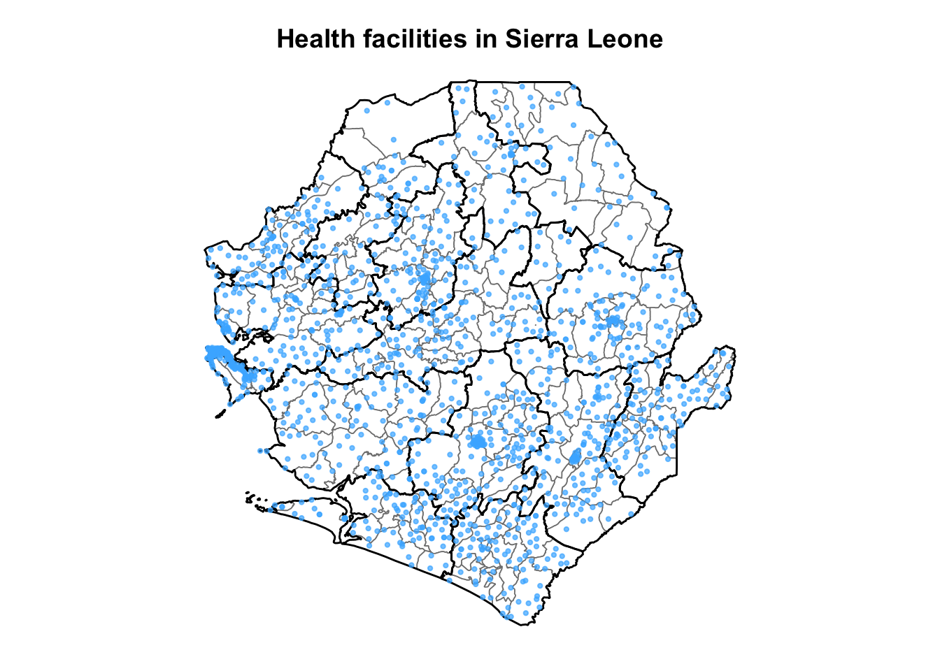
Map saved as: english/outputs/health_facility_locations.png To adapt the code:
- Lines 6-7: Update the map title and output filename
- Lines 11, 12 & 13: Update
fill,color, andsizefor boundary styling - Line 17: Update
color,size, andalphafor health facility points
6.2: Health facilities by type
# Define map title and output filename for facility type map
title_type <- "Health facility types in Sierra Leone"
map_type   <- "health_facility_by_type.png"

# Create health facility type map
facility_type_map <- ggplot2::ggplot() +
  ggplot2::geom_sf(data = df1, fill = "white",
                   color = "gray50", size = 0.3) +
    ggplot2::geom_sf(data = adm2_gdf, fill = NA,
                   color = "black",
                   size = 0.5) +
  ggplot2::geom_point(
    data = facilities_clean,
    ggplot2::aes(x = x, y = y, color = type),
    size = 1, alpha = 0.8
  ) +
  ggplot2::coord_sf() +
  ggplot2::scale_color_brewer(palette = "Set1", name = "Facility Type") +
  ggplot2::theme_void() +
  ggplot2::theme(
    legend.position = "bottom",
    legend.title = ggplot2::element_text(size = 12, face = "bold"),
    legend.text = ggplot2::element_text(size = 10),
    plot.title = ggplot2::element_text(hjust = 0.5, size = 14, face = "bold"),
    plot.margin = ggplot2::margin(10, 10, 10, 10)
  ) +
  ggplot2::labs(title = title_type)

# Print and save the type map
print(facility_type_map)

ggplot2::ggsave(
  filename = file.path(output, map_type),
  plot = facility_type_map,
  width = 10,
  height = 7,
  bg = "white",
  dpi = 300
)

cat("Facility type map saved as:", file.path(output, map_type), "\n")
NoteOutput
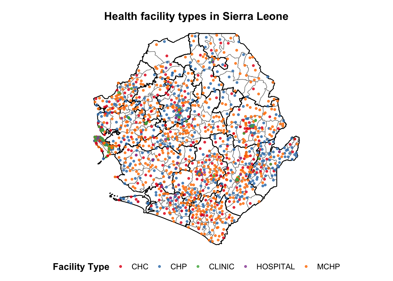
Facility type map saved as: english/outputs/health_facility_by_type.png To adapt the code:
- Lines 6-7: Update the map title and output filename
- Line 15: Replace
typewith the facility type column name - Line 19: Update
palettefor different color schemes
6.3: Specific health facility types
# Define map title and output filename for faceted map
title_facet <- "Health facility distribution by type in Sierra Leone"
map_facet   <- "health_facility_faceted_by_type.png"

# Create faceted map by facility type
faceted_type_map <- ggplot2::ggplot() +
  ggplot2::geom_sf(data = df1, fill = "white",
                   color = "gray50", size = 0.2) +
    ggplot2::geom_sf(data = adm2_gdf, fill = NA,
                   color = "black",
                   size = 0.5) +
  ggplot2::geom_point(
    data = facilities_clean,
    ggplot2::aes(x = x, y = y),
    color = "#47B5FF", size = 1, alpha = 0.7
  ) +
  ggplot2::facet_wrap(~ type) +
  ggplot2::coord_sf() +
  ggplot2::theme_void() +
  ggplot2::theme(
    plot.title = ggplot2::element_text(hjust = 0.5, size = 14, face = "bold"),
    strip.text = ggplot2::element_text(face = "bold", size = 10),
    plot.margin = ggplot2::margin(10, 10, 10, 10)
  ) +
  ggplot2::labs(title = title_facet)

# Print the faceted map
print(faceted_type_map)

# Save the faceted map
ggplot2::ggsave(
  filename = file.path(output, map_facet),
  plot = faceted_type_map,
  width = 12,
  height = 9,
  bg = "white",
  dpi = 300
)

cat("Faceted type map saved as:", file.path(output, map_facet), "\n")
NoteOutput
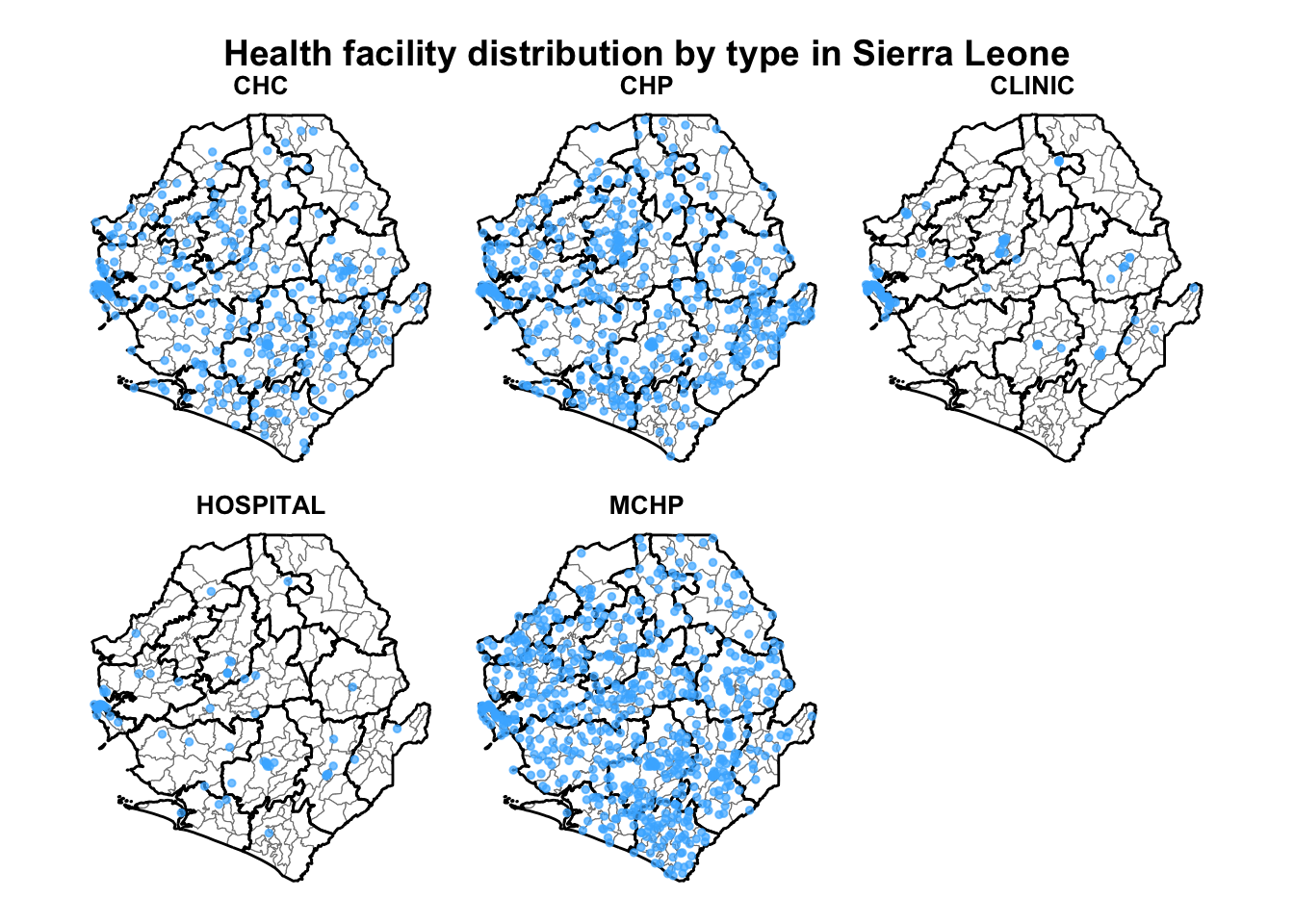
Faceted type map saved as: english/outputs/health_facility_faceted_by_type.png To adapt the code:
- Line 6: Change
"HOSPITAL"to match your desired facility type - Lines 10-11: Update map title and filename accordingly
- Line 20: Update point
colorandsizeas desired
Step 7: Advanced point coordinates visualizations
Point coordinates data can be used to visualize indicators at the facility level in addition to geographic location. The example below uses the merged DHIS2-MFL data obtained through the Fuzzy Matching of Names Across Datasets page of this code library.
7.1: Point coordinates data summary
This examples uses merged DHIS2-MFL data to calculate the test posivity rate for each health facility. Test positivity is the proportion of positive cases out of all cases tested. First we calculate test positivity rate for each health facility per year.
final_dhis2_mfl_integrated <- readRDS(
  here::here(
  "english/data_r/health_facility/final_dhis2_mfl_integrated.rds"))

# Calculate annual summaries for each health facility
annual_summary <- final_dhis2_mfl_integrated |>
  dplyr::group_by(hf_uid, hf, year, lat, long) |>
  dplyr::summarise(
    # Sum tests across all age groups and settings
    total_tests = sum(test_u5 + test_5_14 + test_ov15,
                          na.rm = TRUE),
    # Sum positive tests across all age groups and settings
    positive_tests = sum(conf_u5 + conf_5_14 + conf_ov15,
                             na.rm = TRUE),
    .groups = 'drop') |>
  # Calculate Test Positivity Rate (TPR) as percentage
  dplyr::mutate(
    tpr = base::ifelse(total_tests > 0,
                      (positive_tests / total_tests) * 100,
                      NA_real_)) |>
  # Remove facilities with no tests
  dplyr::filter(total_tests > 0)

# Filter for 2023 only and remove NA/zero-testing facilities
annual_summary_2023 <- annual_summary |>
  dplyr::filter(year == 2023, !is.na(tpr), total_tests > 0,
                !is.na(lat), !is.na(long)) |>
  dplyr::mutate(
    size_category = dplyr::case_when(
      total_tests <= 100 ~ "≤100",
      total_tests <= 500 ~ "101-500",
      total_tests <= 1000 ~ "501-1,000",
      total_tests <= 5000 ~ "1,001-5,000",
      TRUE ~ "5,000+"
    ),
    size_category = factor(size_category,
                          levels = c("≤100", "101-500", "501-1,000",
                                     "1,001-5,000", "5,000+"))
  )
7.2: Single indicator points coordinate visualization
This code plots health facilities by their geographic coordinates and uses the colouring of points to indicate the test positivity value for that facility. For simplicity, this plot shows only 2023 test positivity rates by facility.
map_tpr_2023 <- "health_facility_tpr_2023.png"

tpr_only_2023 <- ggplot2::ggplot() +
  ggplot2::geom_sf(data = df1, fill = "white",
                   color = "gray50", size = 0.3) +
  ggplot2::geom_sf(data = adm2_gdf, fill = NA,
                   color = "black",
                   size = 0.5) +
  ggplot2::geom_point(
    data = annual_summary_2023,
    ggplot2::aes(x = long, y = lat, fill = tpr),
    shape = 21,
    size = 2,
    stroke = 0.5,
    alpha = 0.8
  ) +
  ggplot2::coord_sf() +
  ggplot2::scale_fill_gradientn(
    colors = rev(RColorBrewer::brewer.pal(7, "RdYlBu")),
    limits = c(0, 100),
    name = "Test Positivity Rate (%)",
  ) +
  ggplot2::theme_void() +
  ggplot2::theme(
    legend.position = "right",
    legend.title = ggplot2::element_text(size = 11, face = "bold"),
    legend.text = ggplot2::element_text(size = 10),
    plot.title = ggplot2::element_text(hjust = 0.5, size = 14, face = "bold"),
    plot.margin = ggplot2::margin(10, 10, 10, 10),
    legend.key.size = grid::unit(1, "cm")
  ) +
  ggplot2::labs(title = "Health Facility Test Positivity Rate (2023)")

# Print and save map
print(tpr_only_2023)

ggplot2::ggsave(
  filename = file.path(output, map_tpr_2023),
  plot = tpr_only_2023,
  width = 10,
  height = 7,
  bg = "white",
  dpi = 300
)

cat("2023 TPR map saved as:", file.path(output, map_tpr_2023), "\n")
NoteOutput
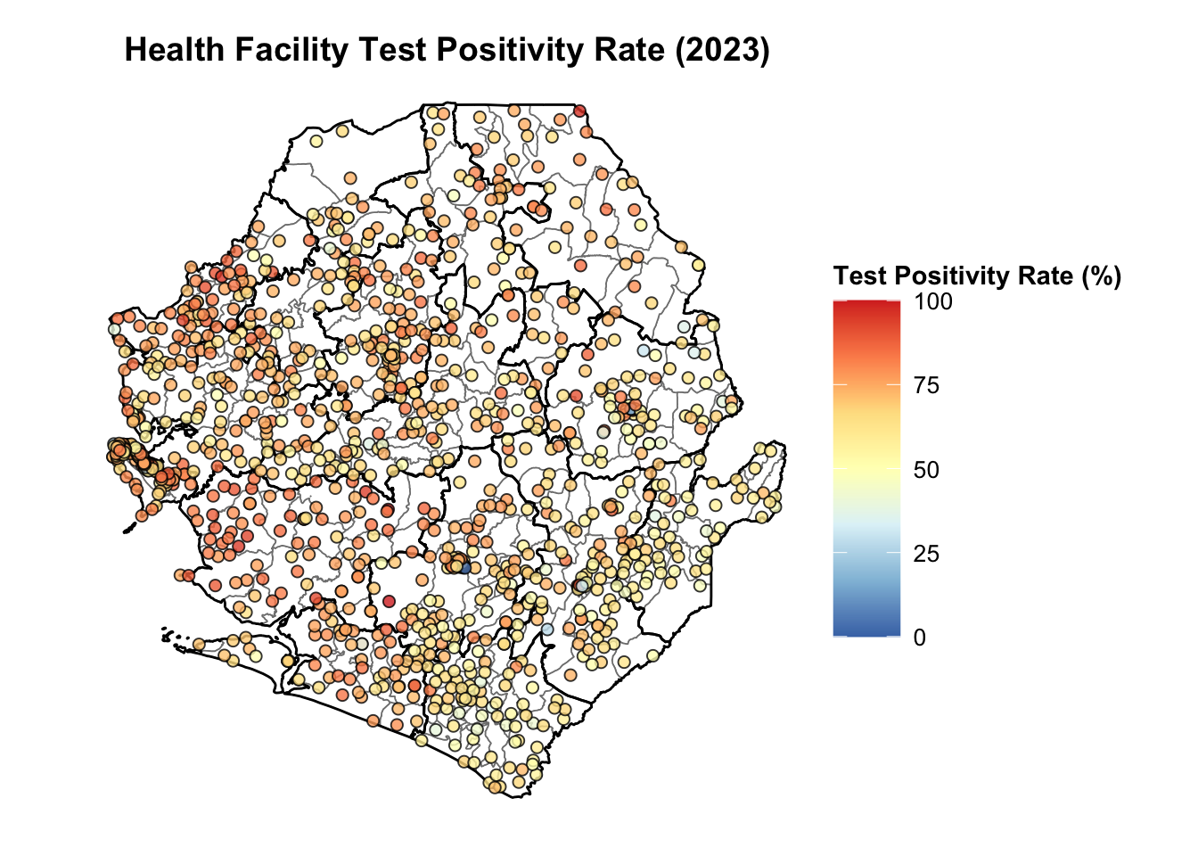
2023 TPR map saved as: english/outputs/health_facility_tpr_2023.png 7.3: Multiple indicator points coordinate visualization
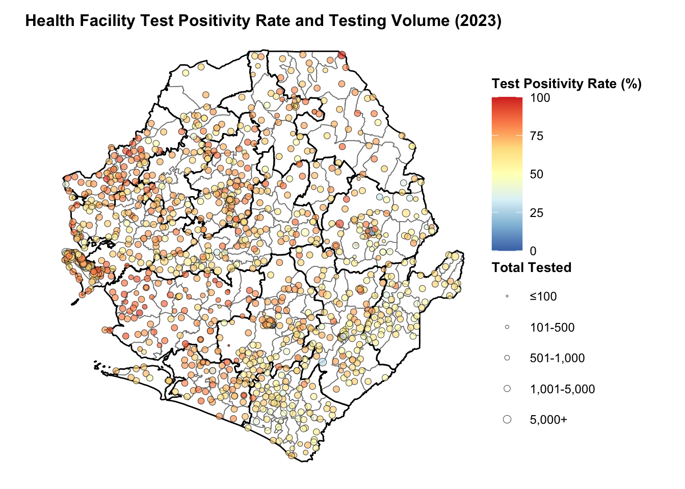
The previous example can be built upon by adding additional plot elements to represent other indicators. For example, the size of each health facilities point can be used to represent testing volume. The code below illustrates this example.
map_tpr_test_2023 <- "health_facility_tpr_test_2023.png"

size_scale <- c("≤50" = 1.5, "51-200" = 2.0, "201-1,000" = 2.5,
                "1,001-5,000" = 3.0, "5,000+" = 3.5)


combined_2023_categorical <- ggplot2::ggplot() +
  ggplot2::geom_sf(data = df1, fill = "white",
                   color = "gray50", size = 0.3) +
  ggplot2::geom_sf(data = adm2_gdf, fill = NA,
                   color = "black",
                   size = 0.5) +
  ggplot2::geom_point(
    data = annual_summary_2023,
    ggplot2::aes(x = long, y = lat,
                 fill = tpr,
                 size = size_category),
    shape = 21,
    stroke = 0.3,  # Thinner stroke
    alpha = 0.7
  ) +
  ggplot2::coord_sf() +
  ggplot2::scale_fill_gradientn(
    colors = rev(RColorBrewer::brewer.pal(7, "RdYlBu")),
    limits = c(0, 100),
    name = "Test Positivity Rate (%)",
    na.value = "grey50"
  ) +
  ggplot2::scale_size_manual(
    name = "Total Tested",
    values = size_scale,
    breaks = c("≤50", "51-200", "201-1,000", "1,001-5,000", "5,000+")
  ) +
  ggplot2::theme_void() +
  ggplot2::theme(
    legend.position = "right",
    legend.title = ggplot2::element_text(size = 10, face = "bold"),
    legend.text = ggplot2::element_text(size = 9),
    plot.title = ggplot2::element_text(hjust = 0.5, size = 12, face = "bold"),
    plot.margin = ggplot2::margin(5, 5, 5, 5),
    legend.key.size = grid::unit(0.8, "cm")
  ) +
  ggplot2::labs(title = "Health Facility Test Positivity Rate and Testing Volume (2023)")

# Print the categorical version
print(combined_2023_categorical)

ggplot2::ggsave(
  filename = file.path(output, map_tpr_test_2023),
  plot = combined_2023_categorical,
  width = 10,
  height = 7,
  bg = "white",
  dpi = 300
)

cat("2023 TPR categorical map saved as:", file.path(output, map_tpr_test_2023), "\n")
NoteOutput
2023 TPR categorical map saved as: english/outputs/health_facility_tpr_test_2023.png Summary
This streamlined workflow outlines steps to visualize health facility coordinates effectively:
Organized file management: Use consistent directory structure and clear variable naming for better code maintainability
Flexible coordinate handling: Support both combined and separate coordinate columns with automatic splitting when needed
Data quality assurance: Validate coordinate ranges and remove invalid entries before mapping
Efficient spatial conversion: Create spatial objects for advanced geographic operations and analysis
Advanced indicator visualization: Use points coordinate data to visualize multiple indicators effectively
Full code
The complete script for mapping health facility coordinates with administrative boundaries is below.
Code
# =============================================================================
# Health facility coordinate mapping and visualization
# =============================================================================
# This script creates comprehensive health facility maps with administrative
# boundaries, showing facility locations and distributions.
# Optimized for SNT (Sub-National Tailoring) processes and health system planning.

# =============================================================================
# Step 1: Install and Load Packages
# =============================================================================

# Check if 'pacman' is installed; install it if missing
if (!requireNamespace("pacman", quietly = TRUE)) {
  install.packages("pacman")
}

# Load all required packages using pacman
pacman::p_load(
  sf,           # for reading and handling spatial data
  readxl,       # for reading Excel files
  readr,        # for reading CSVs
  dplyr,        # for data manipulation
  stringr,      # for string cleaning and formatting
  ggplot2,      # for creating plots
  RColorBrewer, # for color palettes
  scales,       # for formatting scales and labels
  here,         # for cross-platform file paths
  tidyr         # for data reshaping and coordinate splitting
)

# =============================================================================
# Step 2: Load and Prepare Input Data
# =============================================================================

# Define base directories and filenames
shp_dir <- "data/shapefiles/raw"
hf_dir  <- "english/data_r/health_facility"

# Define filenames
shp_file <- "Chiefdom2021.shp"
hf_file  <- "mfl_hfs.xlsx"

# Compose full file paths for data loading
shp_path <- here::here(shp_dir, shp_file)
hf_path  <- here::here(hf_dir, hf_file)

# Load shapefile and transform CRS to WGS84
df1 <- sf::st_read(shp_path, quiet = TRUE) |>
  sf::st_transform(crs = sf::st_crs(4326))

# Load health facility Excel data
df2 <- readxl::read_excel(hf_path)

# =============================================================================
# Step 3: Split Coordinates Column into Latitude and Longitude (if needed)
# This step is only required if longitude and latitude are combined in a single column
# If columns are separate, skip this step
# =============================================================================

# Replace separators (; or space) with a comma
df2$coordinates <- gsub("[; ]+", ",", df2$coordinates)

# Split coordinates column by comma into two columns
df2 <- tidyr::separate(df2, col = "coordinates",
                       into = c("w_lat", "w_long"),
                       sep = ",", convert = TRUE)

df2$x <- df2$w_long
df2$y <- df2$w_lat


# Filter to remove missing or out-of-range coordinates
facilities_clean <- df2[
  !is.na(df2$x) & !is.na(df2$y) &
  df2$x >= -180 & df2$x <= 180 &
  df2$y >= -90 & df2$y <= 90,
]


# =============================================================================
# Step 4: Convert to spatial object
# =============================================================================


facilities_sf <- sf::st_as_sf(
  facilities_clean,
  coords = c("w_long", "w_lat"),
  crs = 4326
)

# =============================================================================
# Step 5: Save Cleaned and Spatial Data
# =============================================================================

# Create output directory
output <- "english/outputs"
dir.create(output, recursive = TRUE, showWarnings = FALSE)

# Define output filenames and paths
hf <- "facilities.csv"
sf <- "facilities_spatial.shp"

hf_path <- file.path(output, hf)
sf_path <- file.path(output, sf)

# Save cleaned data as CSV
write.csv(facilities_clean, hf_path, row.names = FALSE)

# Save spatial data as shapefile
sf::st_write(facilities_sf, sf_path, append = FALSE, quiet = TRUE)

# =============================================================================
# Step 6: Create and Save Health Facility Maps
# =============================================================================

# Define map title and output filename
title <- "Health facilities in Sierra Leone"
map   <- "health_facility_locations.png"

# Create the basic map
facilities_map <- ggplot2::ggplot() +
  ggplot2::geom_sf(data = df1, fill = "white",
                   color = "grey50",
                   size = 0.3) +
  ggplot2::geom_sf(data = adm2_gdf, fill = NA,
                   color = "black",
                   size = 0.5) +
  ggplot2::geom_point(
    data = facilities_clean,
    ggplot2::aes(x = x, y = y),
    color = "#47B5FF", size = 0.8, alpha = 0.7
  ) +
  ggplot2::coord_sf() +
  ggplot2::theme_void() +
  ggplot2::theme(
    plot.title = ggplot2::element_text(hjust = 0.5,
                                       size = 14,
                                       face = "bold"),
    plot.margin = ggplot2::margin(10, 10, 10, 10)
  ) +
  ggplot2::labs(title = title)

# Print and save the map
print(facilities_map)

ggplot2::ggsave(
  filename = file.path(output, map),
  plot = facilities_map,
  width = 10,
  height = 7,
  bg = "white",
  dpi = 300
)


# 6.2: Health facilities by type
# Define map title and output filename for facility type map
title_type <- "Health facility types in Sierra Leone"
map_type   <- "health_facility_by_type.png"

# Create health facility type map
facility_type_map <- ggplot2::ggplot() +
  ggplot2::geom_sf(data = df1, fill = "white",
                   color = "gray50", size = 0.3) +
    ggplot2::geom_sf(data = adm2_gdf, fill = NA,
                   color = "black",
                   size = 0.5) +
  ggplot2::geom_point(
    data = facilities_clean,
    ggplot2::aes(x = x, y = y, color = type),
    size = 1, alpha = 0.8
  ) +
  ggplot2::coord_sf() +
  ggplot2::scale_color_brewer(palette = "Set1", name = "Facility Type") +
  ggplot2::theme_void() +
  ggplot2::theme(
    legend.position = "bottom",
    legend.title = ggplot2::element_text(size = 12, face = "bold"),
    legend.text = ggplot2::element_text(size = 10),
    plot.title = ggplot2::element_text(hjust = 0.5, size = 14, face = "bold"),
    plot.margin = ggplot2::margin(10, 10, 10, 10)
  ) +
  ggplot2::labs(title = title_type)

# Print and save the type map
print(facility_type_map)

ggplot2::ggsave(
  filename = file.path(output, map_type),
  plot = facility_type_map,
  width = 10,
  height = 7,
  bg = "white",
  dpi = 300
)

# 6.3: Specific health facility types
# Define map title and output filename for faceted map
title_facet <- "Health facility distribution by type in Sierra Leone"
map_facet   <- "health_facility_faceted_by_type.png"

# Create faceted map by facility type
faceted_type_map <- ggplot2::ggplot() +
  ggplot2::geom_sf(data = df1, fill = "white",
                   color = "gray50", size = 0.2) +
    ggplot2::geom_sf(data = adm2_gdf, fill = NA,
                   color = "black",
                   size = 0.5) +
  ggplot2::geom_point(
    data = facilities_clean,
    ggplot2::aes(x = x, y = y),
    color = "#47B5FF", size = 1, alpha = 0.7
  ) +
  ggplot2::facet_wrap(~ type) +
  ggplot2::coord_sf() +
  ggplot2::theme_void() +
  ggplot2::theme(
    plot.title = ggplot2::element_text(hjust = 0.5, size = 14, face = "bold"),
    strip.text = ggplot2::element_text(face = "bold", size = 10),
    plot.margin = ggplot2::margin(10, 10, 10, 10)
  ) +
  ggplot2::labs(title = title_facet)

# Print the faceted map
print(faceted_type_map)

# Save the faceted map
ggplot2::ggsave(
  filename = file.path(output, map_facet),
  plot = faceted_type_map,
  width = 12,
  height = 9,
  bg = "white",
  dpi = 300
)

# =============================================================================
# Step 7: Advanced plotting
# =============================================================================


final_dhis2_mfl_integrated <- readRDS(
  here::here(
  "english/data_r/health_facility/final_dhis2_mfl_integrated.rds"))

# Calculate annual summaries for each health facility
annual_summary <- final_dhis2_mfl_integrated |>
  dplyr::group_by(hf_uid, hf, year, lat, long) |>
  dplyr::summarise(
    # Sum tests across all age groups and settings
    total_tests = sum(test_u5 + test_5_14 + test_ov15,
                          na.rm = TRUE),
    # Sum positive tests across all age groups and settings
    positive_tests = sum(conf_u5 + conf_5_14 + conf_ov15,
                             na.rm = TRUE),
    .groups = 'drop') |>
  # Calculate Test Positivity Rate (TPR) as percentage
  dplyr::mutate(
    tpr = base::ifelse(total_tests > 0,
                      (positive_tests / total_tests) * 100,
                      NA_real_)) |>
  # Remove facilities with no tests
  dplyr::filter(total_tests > 0)

# Filter for 2023 only and remove NA/zero-testing facilities
annual_summary_2023 <- annual_summary |>
  dplyr::filter(year == 2023, !is.na(tpr), total_tests > 0,
                !is.na(lat), !is.na(long)) |>
  dplyr::mutate(
    size_category = dplyr::case_when(
      total_tests <= 100 ~ "≤100",
      total_tests <= 500 ~ "101-500",
      total_tests <= 1000 ~ "501-1,000",
      total_tests <= 5000 ~ "1,001-5,000",
      TRUE ~ "5,000+"
    ),
    size_category = factor(size_category,
                          levels = c("≤100", "101-500", "501-1,000",
                                     "1,001-5,000", "5,000+"))
  )

map_tpr_2023 <- "health_facility_tpr_2023.png"

tpr_only_2023 <- ggplot2::ggplot() +
  ggplot2::geom_sf(data = df1, fill = "white",
                   color = "gray50", size = 0.3) +
  ggplot2::geom_sf(data = adm2_gdf, fill = NA,
                   color = "black",
                   size = 0.5) +
  ggplot2::geom_point(
    data = annual_summary_2023,
    ggplot2::aes(x = long, y = lat, fill = tpr),
    shape = 21,
    size = 2,
    stroke = 0.5,
    alpha = 0.8
  ) +
  ggplot2::coord_sf() +
  ggplot2::scale_fill_gradientn(
    colors = rev(RColorBrewer::brewer.pal(7, "RdYlBu")),
    limits = c(0, 100),
    name = "Test Positivity Rate (%)",
  ) +
  ggplot2::theme_void() +
  ggplot2::theme(
    legend.position = "right",
    legend.title = ggplot2::element_text(size = 11, face = "bold"),
    legend.text = ggplot2::element_text(size = 10),
    plot.title = ggplot2::element_text(hjust = 0.5, size = 14, face = "bold"),
    plot.margin = ggplot2::margin(10, 10, 10, 10),
    legend.key.size = grid::unit(1, "cm")
  ) +
  ggplot2::labs(title = "Health Facility Test Positivity Rate (2023)")

# Print and save map
print(tpr_only_2023)

ggplot2::ggsave(
  filename = file.path(output, map_tpr_2023),
  plot = tpr_only_2023,
  width = 10,
  height = 7,
  bg = "white",
  dpi = 300
)

cat("2023 TPR map saved as:", file.path(output, map_tpr_2023), "\n")

map_tpr_test_2023 <- "health_facility_tpr_test_2023.png"

size_scale <- c("≤50" = 1.5, "51-200" = 2.0, "201-1,000" = 2.5,
                "1,001-5,000" = 3.0, "5,000+" = 3.5)


combined_2023_categorical <- ggplot2::ggplot() +
  ggplot2::geom_sf(data = df1, fill = "white",
                   color = "gray50", size = 0.3) +
  ggplot2::geom_sf(data = adm2_gdf, fill = NA,
                   color = "black",
                   size = 0.5) +
  ggplot2::geom_point(
    data = annual_summary_2023,
    ggplot2::aes(x = long, y = lat,
                 fill = tpr,
                 size = size_category),
    shape = 21,
    stroke = 0.3,  # Thinner stroke
    alpha = 0.7
  ) +
  ggplot2::coord_sf() +
  ggplot2::scale_fill_gradientn(
    colors = rev(RColorBrewer::brewer.pal(7, "RdYlBu")),
    limits = c(0, 100),
    name = "Test Positivity Rate (%)",
    na.value = "grey50"
  ) +
  ggplot2::scale_size_manual(
    name = "Total RDT Tests",
    values = size_scale,
    breaks = c("≤50", "51-200", "201-1,000", "1,001-5,000", "5,000+")
  ) +
  ggplot2::theme_void() +
  ggplot2::theme(
    legend.position = "right",
    legend.title = ggplot2::element_text(size = 10, face = "bold"),
    legend.text = ggplot2::element_text(size = 9),
    plot.title = ggplot2::element_text(hjust = 0.5, size = 12, face = "bold"),
    plot.margin = ggplot2::margin(5, 5, 5, 5),
    legend.key.size = grid::unit(0.8, "cm")
  ) +
  ggplot2::labs(title = "Health Facility Test Positivity Rate and Testing Volume (2023)")

# Print the categorical version
print(combined_2023_categorical)

ggplot2::ggsave(
  filename = file.path(output, map_tpr_test_2023),
  plot = combined_2023_categorical,
  width = 10,
  height = 7,
  bg = "white",
  dpi = 300
)

cat("2023 TPR categorical map saved as:", file.path(output, map_tpr_test_2023), "\n")