#===============================================================================
# Step 1: Set-Up and Download DHS data
#===============================================================================
# Install pacman only if it's not already installed
if (!requireNamespace("pacman", quietly = TRUE)) {
  install.packages("pacman")
}

# install or load relevant packages
pacman::p_load(
  rdhs,      # for downloading dhs data
  tidyverse, # core tidy tools (includes dplyr, tidyr, readr, etc.)
  haven,     # read and write various data formats (stata)
  httr,      # download files from web (GET, write_disk)
  rio,       # importing data
  here,      # relative file pathways
  data.table,# is an excellent extension of the data.frame class
  fs,        # handle file paths
  purrr,     # iterate over lists (map, walk, etc.)
  rlang,     # for tidy evaluation and error messaging
  survey,    # analyzing data from complex surveys
  sf,        # Support for simple feature access, a standardized way
             # to encode and analyze spatial vector data
  tmap,      # drawing thematic maps
  knitr      # Make table
)
# Create a complex survey design object
 svydesign.fun <- function(filename){
## Create a Survey Design Object
  survey::svydesign(id = ~id,
            strata = ~strate, nest = T,
            weights = ~wt, data = filename)
 }

# Computes survey-weighted proportions
 result.prop <- function(var, var1, design) {
  p_est <- survey::svyby(formula = make.formula(var), by = make.formula(var1),
                       FUN = svymean, design, levels = 0.95, vartype = "ci",
                       na.rm = T, influence = TRUE)
 }

# Estimation functions
estim_prop <- function(df, col, by){
  svy_mal <- svydesign.fun(df)
  region_est <- result.prop(col, by, design = svy_mal)
}
# Set DHS configuration
rdhs::set_rdhs_config(
email = "my_email_address@gmail.com",
project = "SNT for SL",
config_path = "dhs.json",
cache_path = here::here("1.6_health_systems/1.6a_dhs"),
data_frame = "data.table::as.data.table",
global = FALSE,
password_prompt = TRUE,
verbose_setup = TRUE,
timeout = 120,
verbose_download = TRUE
)
# Get the 2013 and 2019 SL DHS and MIS dataset filenames
data_filename <- rdhs::dhs_datasets(
countryIds = "SL",
surveyYear = c("2016", "2019"),
fileType = c("KR", "PR"),
surveyType = c("DHS", "MIS"),
fileFormat = "FLAT"
) |>
dplyr::group_by(DatasetType, CountryName, FileType) |>
dplyr::distinct() |>
dplyr::pull(FileName)
# Download the DHS datasets
rdhs::get_datasets(
dataset_filenames = data_filename,
download_option = "rds",
output_dir_root = here::here("1.6_health_systems/1.6a_dhs/raw"),
clear_cache = TRUE
)
#===============================================================================
# Step 2: Extract Children with Recent (Malaria) Fever
#===============================================================================
# Import and process DHS KR files for 2013 and 2019
mis_kr_2016 <- readRDS(
here::here("1.6_health_systems/1.6a_dhs/raw/SLKR73FL.rds")) |>
haven::zap_labels() |> # remove labels to make merging easier
dplyr::select(
caseid, v001, v002, v003, v007, v012, v022, v021,
v024, v101, v005, b5, b8, b19, h22, h32a:h32y
)
dhs_kr_2019 <- readRDS(
here::here("1.6_health_systems/1.6a_dhs/raw/SLKR7AFL.rds")) |>
haven::zap_labels() |> # remove labels to make merging easier
dplyr::select(
caseid, v001, v002, v003, v007, v012, v022, v021,
v024, v101, v005, b5, b8, b19, h22, h32a:h32y
)
# Combine both survey rounds
dhs_kr <- dplyr::bind_rows(mis_kr_2016, dhs_kr_2019)
# Process each dataset in the list
dhs <- dhs_kr |>
# Create helper variables: admin-1, weights, strata,
# cluster ID, year, fever indicator
dplyr::mutate(
adm1 = ifelse(is.na(v024), v101, v024),
wt = v005 / 1000000, strate = v022, id = v021,
year = v007,
ml_fever = ifelse(h22 == 1, 1, 0)) |>
# Recode admin-1 region codes to consistent readable region names (year-dependent)
dplyr::mutate(
adm1 = dplyr::case_when(
adm1 == 1 ~ "eastern",
adm1 == 2 ~ "northern",
adm1 == 3 & year == 2019 ~ "north western",
adm1 == 3 & year == 2016 ~ "southern",
adm1 == 4 & year == 2019 ~ "southern",
adm1 == 4 & year == 2016 ~ "western",
adm1 == 5 ~ "western",
TRUE ~ NA_character_
)) |>
# Filter to include only living children under age 5 with valid fever responses
dplyr::filter(
b5 == 1 & b19 < 60 & h22 != 8)
# File with only children with fever
dhs_fever <- dhs |>
dplyr::filter(ml_fever == 1)
# Filter to fever cases and summarize by admin-1
data_output = dhs |>
dplyr::filter(ml_fever == 1) |>
dplyr::group_by(adm1) |>
dplyr::summarise(ml_fever = sum(ml_fever, na.rm = T))
# Display summary table with number of fevers by admin-1
knitr::kable(data_output, caption = "Number of fevers by admin-1 level")
# Import and process MIS PR files for 2013 and 2019
mis_pr_2016 <- readRDS(here::here("1.6_health_systems/1.6a_dhs/raw/SLPR73FL.rds")) |>
  haven::zap_labels() |> # remove labels to make merging easier
  dplyr::select(
    v001 = hv001, v002 = hv002, v007 = hv007, hv103,
    hv042, hc1, rdt = hml35)

dhs_pr_2019 <- readRDS(here::here("1.6_health_systems/1.6a_dhs/raw/SLPR7AFL.rds")) |>
  haven::zap_labels() |> # remove labels to make merging easier
  dplyr::select(
    v001 = hv001, v002 = hv002, v007 = hv007, hv103,
    hv042, hc1, rdt = hml35)

# Combine both survey rounds
dhs_pr <- dplyr::bind_rows(mis_pr_2016, mis_pr_2016)

# From the PR file, extract children under 5 who are eligible and RDT positive
data_pr <- dhs_pr |>
  dplyr::filter(
    hv042 == 1 & hv103 == 1 & hc1 %in% c(6:59) & rdt == 1) |>
  dplyr::select(-hv042, -hv103, -hc1)

# Merge fever data with RDT-positive data by cluster, household, and survey year
data_pr_kr <- dhs_fever |>
    dplyr::left_join(
      data_pr, by = c("v001", "v002", "v007"),
      relationship = "many-to-many") |>
    dplyr::filter(rdt == 1) |>
    dplyr::select(-dplyr::starts_with(".id"))

# Group by admin-1 and sum number of RDT-positive children
data_output_rdt = data_pr_kr |>
  dplyr::group_by(adm1) |>
  dplyr::summarise(rdt = sum(rdt, na.rm = T))

# Display the result in a formatted table
knitr::kable(data_output_rdt,
             caption = "Number of RDT-positive fevers by admin-1")
#===============================================================================
# Step 3: Assign Recent Fevers to Source of Treatment
#===============================================================================
dhs_care_seeking <- dhs |>
  # Filter by key factors (child had a fever in last two weeks: h22)
  dplyr::filter(ml_fever == 1) |>

  # Assigning each child to public, private and no care-seeking
  dplyr::mutate(
    ml_fever_pub = rowSums(
      dplyr::across(
        c(
          h32a, h32b, h32c, h32d, h32e,
          h32f, h32g, h32h, h32i
        )), na.rm = TRUE),

    ml_fever_priv = rowSums(
      dplyr::across(
        c(
          h32j, h32k, h32l, h32m, h32n,
          h32o, h32p, h32q, h32r, h32s,
          h32t, h32u, h32v, h32w, h32x
        )), na.rm = TRUE),

    pub = ifelse(ml_fever_pub > 0, 1, 0),
    priv = ifelse(ml_fever_priv > 0, 1, 0),
    pub = ifelse(pub == 1 & priv == 1, 1, pub),
    no_treat = ifelse(h32y == 0, 0, 1)
  )
#===============================================================================
# Step 4: Estimate Treatment-Seeking Rates by Sector at Admin-1 Level
#===============================================================================
# Define indicators
vars <- c("pub", "priv", "no_treat")

# Handle single PSU strata
options(survey.lonely.psu = "adjust")

# Process each dataset in dhs file
data_fever_care <- dhs_care_seeking |>
  # Add a year column
  dplyr::mutate(year = v007) |>
  # Compute proportions for each indicator
  estim_prop(col = vars, by = c("adm1", "year")) |>
  # rename columns, and format
  dplyr::rename(adm1 = 1, year = 2) |>
  dplyr::select(adm1, year, pub, priv, no_treat) |>
  dplyr::mutate(
    pub = round(pub, 2),
    priv = round(priv, 2),
    no_treat = round(no_treat, 2),
    year = as.numeric(year)
  )

# Reset row name
rownames(data_fever_care) <- NULL
#===============================================================================
# Step 5: Visualize Treatment-Seeking Rates by Sector
#===============================================================================
# Import the shapefile using st_read
shp <- readRDS(
here::here("01_foundational/1a_administrative_boundaries",
"1ai_adm3", "sle_adm1_shp.rds")
) |> sf::st_as_sf()
# Pivot the table in long format to have all indicators in a single column
data_care_shp <- data_fever_care |>
tidyr::pivot_longer(cols = c("pub", "priv", "no_treat"),
names_to = "Sectors",
values_to = "values") |>
dplyr::mutate(
Sectors = dplyr::recode(Sectors,
"pub" = "Public care seeking",
"priv" = "Private care seeking",
"no_treat" = "No care seeking"
)
)
# Merge shapefile with care-seeking date
dhs_shp_region <- shp |>
dplyr::left_join(data_care_shp, by = c("adm1"),
relationship = "many-to-many")
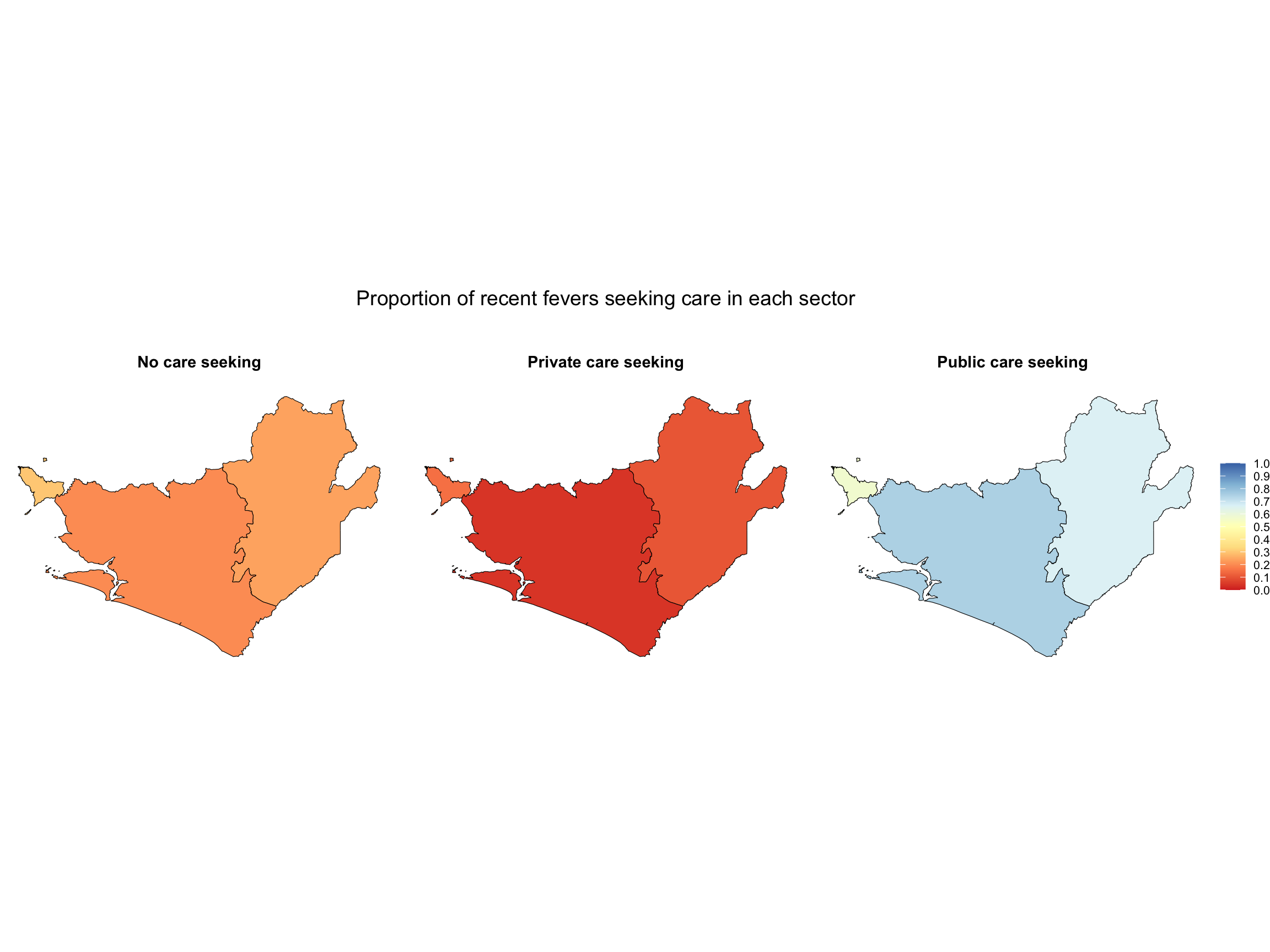
# Create a map to viualize the indicators
g <- dhs_shp_region |>
dplyr::filter(year == 2019) |>
ggplot2::ggplot() +
ggplot2::geom_sf(aes(fill = values), color = "black", size = 0.2) +
ggplot2::facet_wrap(~ Sectors, nrow = 1) +
ggplot2::scale_fill_distiller(
palette = "RdYlBu",
limits = c(0, 1),
breaks = seq(0, 1, by = 0.1),
direction = 1,
na.value = "transparent",
name = NULL
) +
ggplot2::theme_void() +
ggplot2::theme(
legend.position = "right",
legend.title = ggplot2::element_text(size = 10),
legend.text = ggplot2::element_text(size = 8),
panel.grid = ggplot2::element_blank(),
strip.background = ggplot2::element_blank(),
strip.text = ggplot2::element_text(
face = "bold", size = 11, margin = ggplot2::margin(b = 10)),
strip.placement = "outside",
plot.title = ggplot2::element_text(hjust = 0.5, size = 14)
) +
ggplot2::labs(title = "Proportion of recent fevers seeking care in each sector\n\n")
# plot
g
# Save to PNG
ggplot2::ggsave(
filename = here::here("03_output/3a_figures",
"prop_recent_fevers_seeking_care_in_each_sector.png"),
plot = g, width = 10, height = 6, dpi = 300)
#===============================================================================
# Step 6: Estimate Values for Years Without Surveys
#===============================================================================
# Import Guinea treatment seeking rate file
data_inter <- read.csv(here::here("1.6_health_systems/misc/GN_treatment_seeking.csv"))
# Define the target years you want in the final dataset
target_years <- c(2018, 2019, 2020, 2021, 2022, 2023)
# Expand the dataset for all admin × year combinations
df_full <- expand.grid(
adm1 = unique(data_inter$adm1),
year = target_years
) |>
dplyr::left_join(data_inter, by = c("adm1", "year")) |>
dplyr::arrange(adm1, year)
# Fill missing values using last observation carried forward within each admin
df_filled <- df_full |>
dplyr::group_by(adm1) |>
tidyr::fill(pub, priv, no_treat, .direction = "down") |>
dplyr::ungroup()
# Pivot the table in long format to have all indicators in a single column
medfever_dhs_fitted_all_long <- df_filled |>
tidyr::pivot_longer(
cols = c("pub", "priv", "no_treat"),
names_to = "Sectors",
values_to = "Proportion"
) |>
dplyr::mutate(
Sectors = dplyr::recode(Sectors,
"pub" = "Public care seeking",
"priv" = "Private care seeking",
"no_treat" = "No care seeking"
)
)
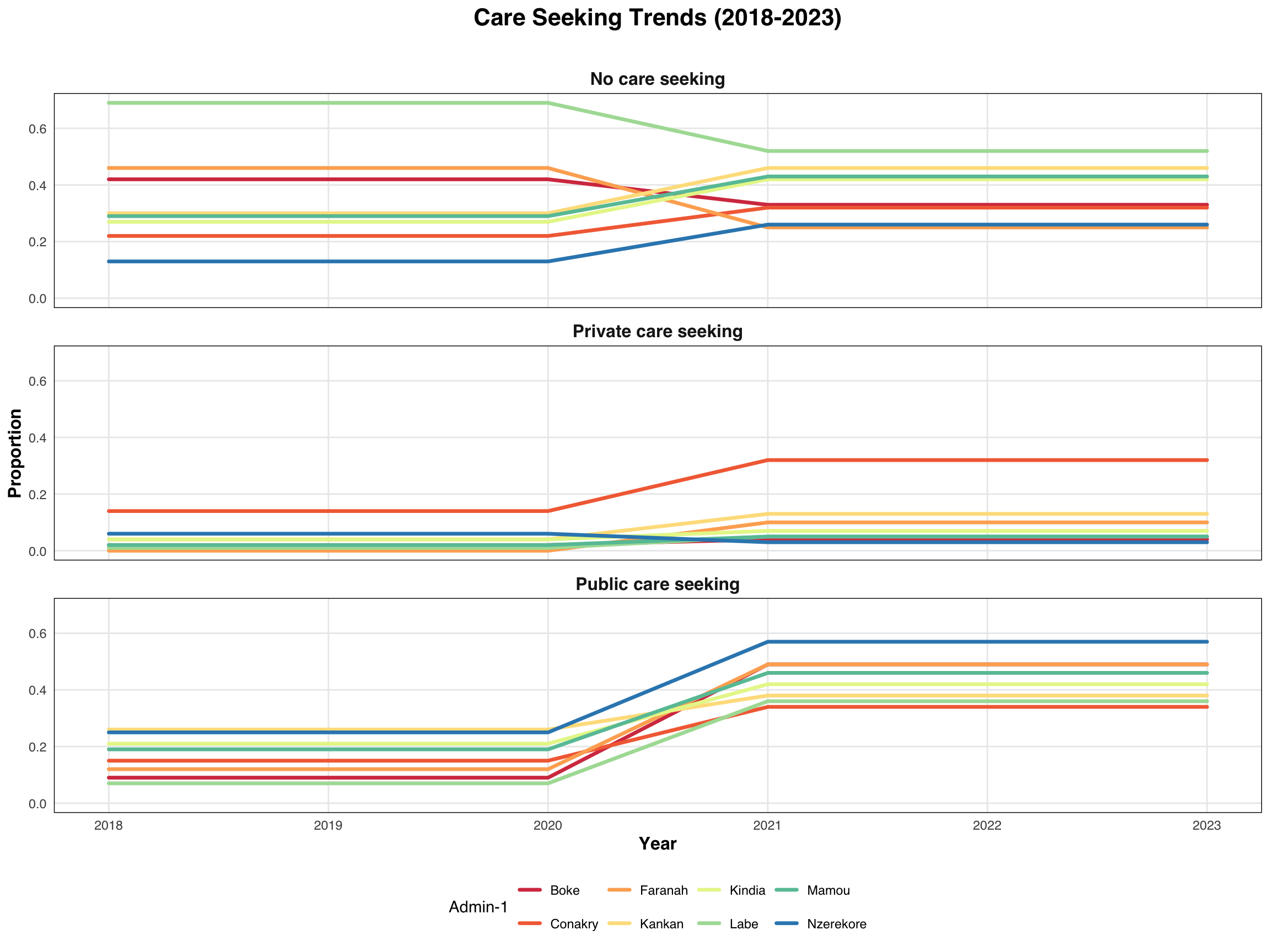
# Visualizing indicators using ggplot2
p <- medfever_dhs_fitted_all_long |>
ggplot2::ggplot(
ggplot2::aes(x = year, y = Proportion,
group = adm1, color = factor(adm1))) +
ggplot2::geom_line(linewidth = 1.2, lineend = "round") +
ggplot2::scale_color_brewer(palette = "Spectral") +
ggplot2::facet_wrap(~ Sectors, ncol = 1) +
ggplot2::theme_minimal() +
ggplot2::labs(title = "Care Seeking Trends (2018-2023)\n",
x = "Year",
y = "Proportion",
color = "Admin-1") +
ggplot2::theme(
text = ggplot2::element_text(family = "sans"),
plot.title = ggplot2::element_text(hjust = 0.5, face = "bold", size = 16),
strip.text = ggplot2::element_text(face = "bold", size = 12),
panel.grid.minor = ggplot2::element_blank(),
panel.border = ggplot2::element_rect(color = "black", fill = NA, size = 0.5),
axis.title = ggplot2::element_text(size = 12, face = "bold"),
legend.position = "bottom"
)
# Print output
p
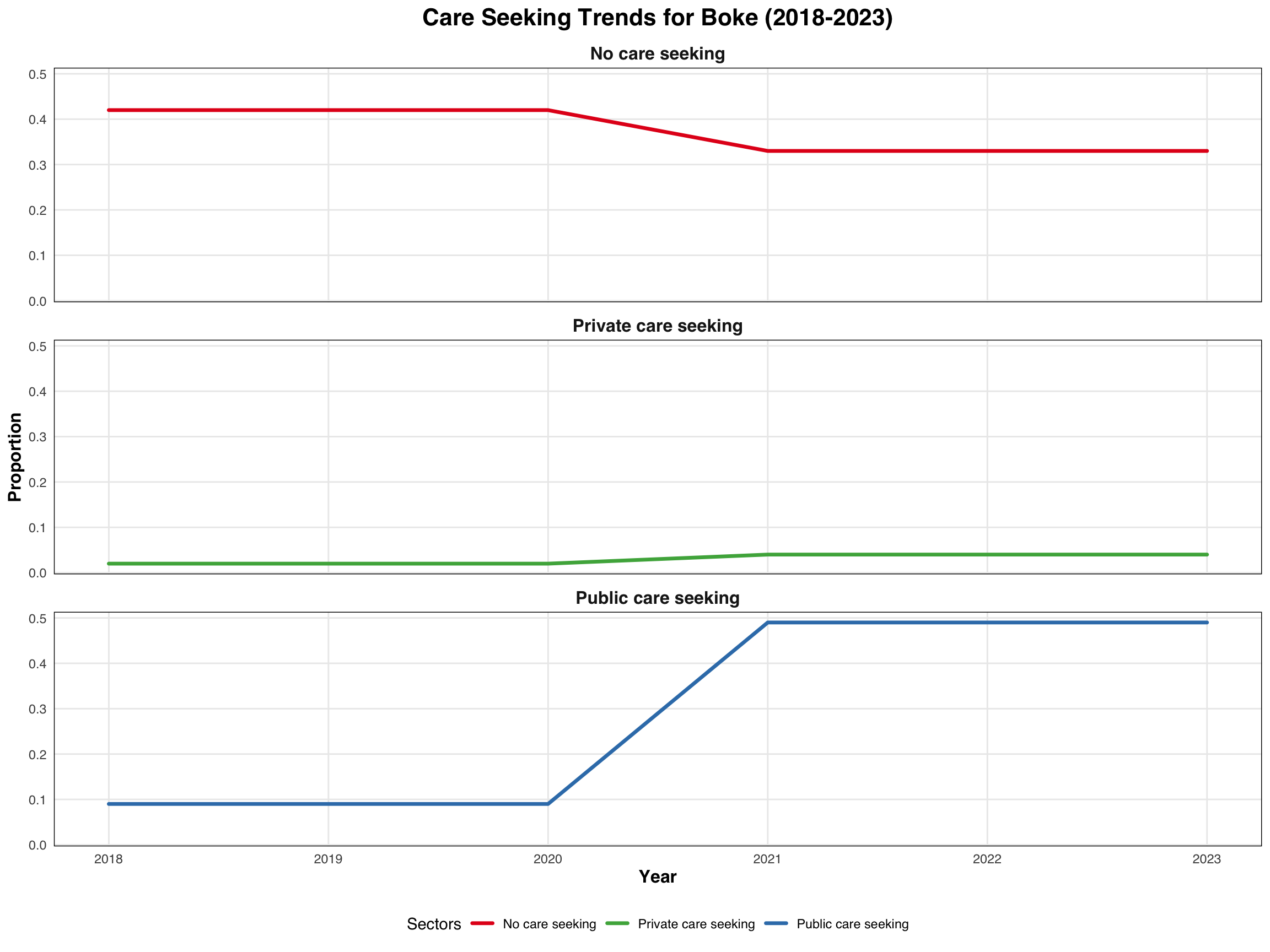
# Visualizing indicators using ggplot2
p1 <- medfever_dhs_fitted_all_long |>
dplyr::filter(adm1 == "Boke") |>
ggplot2::ggplot(
ggplot2::aes(x = year, y = Proportion, color = Sectors)) +
ggplot2::geom_line(size = 1.2, lineend = "round") +
ggplot2::scale_color_manual(values = c("No care seeking" = "#E41A1C",
"Private care seeking" = "#4DAF4A",
"Public care seeking" = "#377EB8")) +
ggplot2::facet_wrap(~ Sectors, ncol = 1) +
ggplot2::theme_minimal() +
ggplot2::labs(title = "Care Seeking Trends for Boke (2018-2023)",
x = "Year",
y = "Proportion",
color = "Sectors") +
ggplot2::theme(
text = ggplot2::element_text(family = "sans"),
plot.title = ggplot2::element_text(hjust = 0.5, face = "bold", size = 16),
strip.text = ggplot2::element_text(face = "bold", size = 12),
panel.grid.minor = ggplot2::element_blank(),
panel.border = ggplot2::element_rect(color = "black", fill = NA, size = 0.5),
axis.title = ggplot2::element_text(size = 12, face = "bold"),
legend.position = "bottom"
)
# Print output
p1
# Save to PNG
ggplot2::ggsave(
filename = here::here("03_output/3a_figures",
"care_seeking_trends_2018-2023.png"),
plot = p, width = 10, height = 6, dpi = 300)
# Save to PNG
ggplot2::ggsave(
filename = here::here("03_output/3a_figures",
"boke_care_seeking_trends_2018-2023.png"),
plot = p1, width = 10, height = 6, dpi = 300)
# Define target years for interpolation
target_years <- c(2019, 2020, 2022, 2023)
# Initialize an empty list to store interpolated results
interpolated_data <- list()
# Loop through each admin-1 (adm1)
for (reg in unique(data_inter$adm1)) {
# Subset data for the current region
reg_data <- data_inter[data_inter$adm1 == reg, ]
# Interpolate each variable (pub, priv, no.treat) using approx()
interp_pub <- approx(reg_data$year, reg_data$pub,
xout = target_years, rule = 2)$y
interp_priv <- approx(reg_data$year, reg_data$priv,
xout = target_years, rule = 2)$y
interp_notrt <- approx(reg_data$year, reg_data$no_treat,
xout = target_years, rule = 2)$y
# Combine into a data frame for this region
reg_result <- data.frame(
adm1 = reg,
year = target_years,
pub = round(interp_pub, 2),
priv = round(interp_priv, 2),
no_treat = round(interp_notrt, 2)
)
# Append to the list
interpolated_data[[reg]] <- reg_result
}
# Combine all regions into a single data frame
medfever_dhs_interp_finale <- dplyr::bind_rows(interpolated_data) |>
# bind all years in one file
dplyr::bind_rows(data_inter)
# Pivot the table in long format to have all indicators in a single column
medfever_dhs_inter_long <- medfever_dhs_interp_finale |>
tidyr::pivot_longer(cols = c("pub", "priv", "no_treat"),
names_to = "Sectors",
values_to = "Proportion") |>
dplyr::mutate(
Sectors = dplyr::recode(Sectors,
"pub" = "Public care seeking",
"priv" = "Private care seeking",
"no_treat" = "No care seeking"
)
)
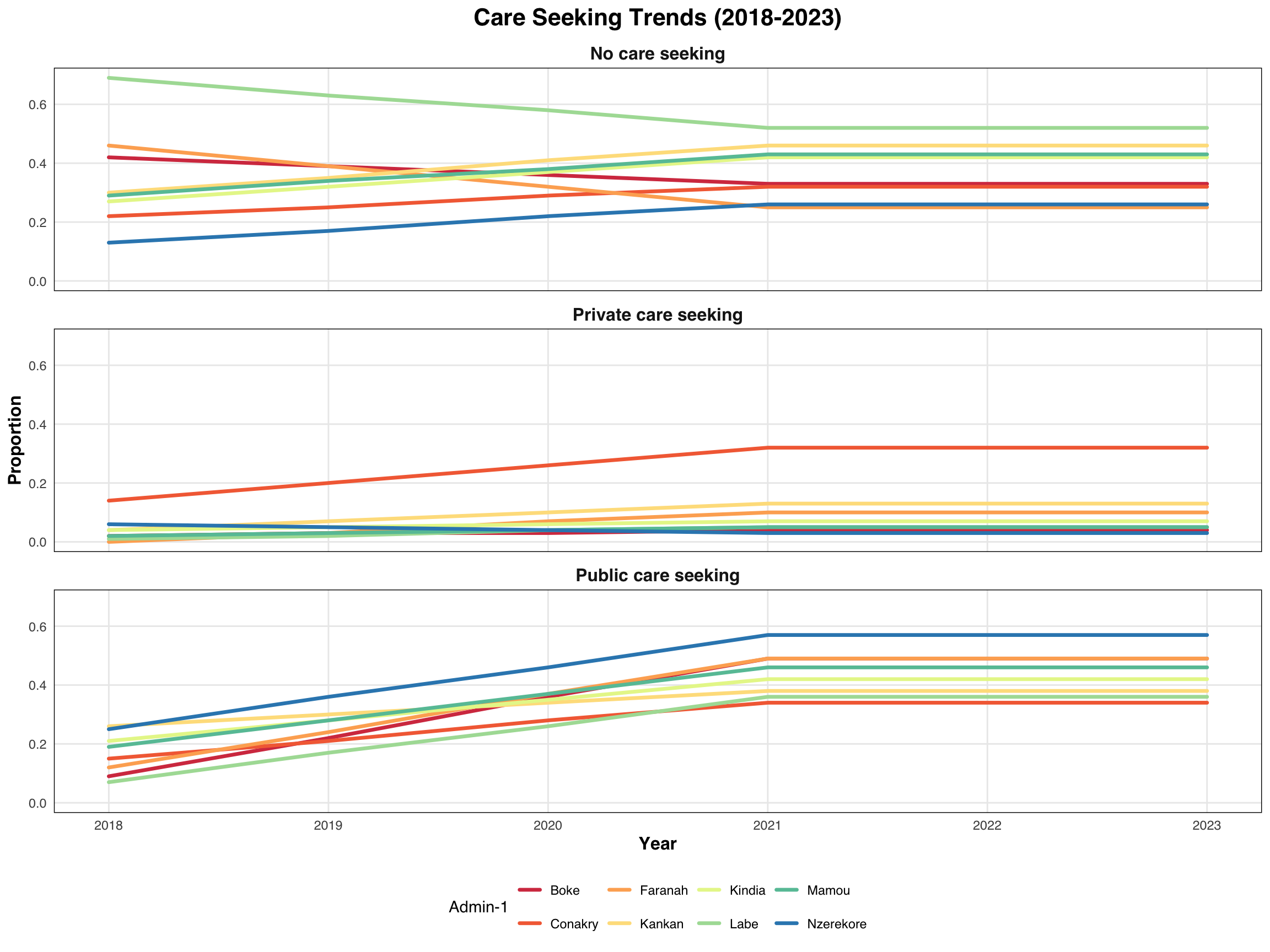
# Visualizing indicators using ggplot2
p2 <- medfever_dhs_inter_long |>
ggplot2::ggplot(
ggplot2::aes(x = year, y = Proportion,
group = adm1, color = factor(adm1))) +
ggplot2::geom_line(size = 1.2, lineend = "round") +
ggplot2::scale_color_brewer(palette = "Spectral") +
ggplot2::facet_wrap(~ Sectors, ncol = 1) +
ggplot2::theme_minimal() +
ggplot2::labs(title = "Care Seeking Trends (2018-2023)",
x = "Year",
y = "Proportion",
color = "Admin-1") +
ggplot2::theme(
text = ggplot2::element_text(family = "sans"),
plot.title = ggplot2::element_text(hjust = 0.5, face = "bold", size = 16),
strip.text = ggplot2::element_text(face = "bold", size = 12),
panel.grid.minor = ggplot2::element_blank(),
panel.border = ggplot2::element_rect(color = "black", fill = NA, size = 0.5),
axis.title = ggplot2::element_text(size = 12, face = "bold"),
legend.position = "bottom"
)
# Print output
p2
# Save to PNG
ggplot2::ggsave(
filename = here::here("03_output/3a_figures",
"care_seeking_trends_2018-2023.png"),
plot = p, width = 10, height = 6, dpi = 300)
#===============================================================================
# Step 7: Save the Output
#===============================================================================
# set up output path
save_path <- here::here("1.6_health_systems/1.6a_dhs/processed")
# save to csv
rio::export(data_fever_care,
here::here(save_path, "care_seeking_data.csv"))
# save to csv
rio::export(medfever_dhs_inter_long,
here::here(save_path, "medfever_dhs_interp.csv"))
# save to csv
rio::export(medfever_dhs_fitted_all_long,
here::here(save_path, "medfever_DHS_linear.csv"))