# Check if 'pacman' is installed; install it if missing
if (!requireNamespace("pacman", quietly = TRUE)) {
  install.packages("pacman")
}

# Load all required packages using pacman
pacman::p_load(
  sf,           # for reading and handling shapefiles
  rio,          # for importing Excel files (replaces readxl)
  dplyr,        # for data manipulation
  stringr,      # for string cleaning and formatting
  ggplot2,      # for creating plots
  cli,          # for styled console output
  here          # for cross-platform file paths
)

# sntutils has a number of useful helper functions for data
# management and cleaning
if (!requireNamespace("sntutils", quietly = TRUE)) {
  devtools::install_github("ahadi-analytics/sntutils")
}

# for parsing coordinates
if (!requireNamespace("parzer", quietly = TRUE)) {
  remotes::install_github("ropensci/parzer")
}Merging shapefiles with tabular data
Intermediate
Overview
In SNT, the spatial dimension is central because the entire process is designed to support tailored assessments and recommendations at subnational levels. The aim is to reflect local heterogeneities in malaria transmission, intervention coverage, and health system capacity. To do this, data must be accurately linked to geographic units like districts or chiefdoms. Every core input, from PfPR estimates and routine surveillance indicators to environmental and campaign data, is tied to place. Our ability to stratify burden, assess program performance, and prioritize actions depends on clean and consistent spatial linkage.
Merging tabular data with spatial boundaries aligns values such as incidence, coverage, or risk classifications with the correct administrative units. This process enables mapping, stratification, and decision-making. Many SNT workflow steps depend on spatial merging: modeled surfaces such as PfPR and environmental covariates overlay with administrative boundaries during stratification; routine indicators from DHIS2 join to district shapefiles for burden analysis; campaign data link to geographic areas to identify coverage gaps. A consistent spatial structure ensures that data from different sources integrate properly, supports alignment across inputs, and produces maps, summaries, and targeting outputs for program use.
Shapefiles serve as the foundation for all SNT process components, requiring reliable methods to join them with other datasets. Differences in naming, formatting, or coordinate precision often cause failed or inaccurate merges. This section demonstrates how to prepare datasets for joining, select appropriate join methods, and validate results. These techniques form the backbone of spatial analysis workflows that analysts will reference throughout the code library.
TipMore on spatial data
For background information on shapefiles and links to all the spatial data content in the SNT code library, including rasters and point data, please visit Spatial data overview.
NoteObjectives
- Integrate spatial and tabular data using attribute-based and coordinate-based joining methods
- Resolve naming inconsistencies, coordinate issues, and CRS misalignment through systematic validation
- Apply diagnostic checks to ensure complete and accurate spatial linkage
- Handle edge cases including buffered joins, DMS conversion, and boundary precision issues
- Validate results using visualization techniques
- Save outputs for subsequent analysis
Understanding Spatial Joins
Before analyzing or visualizing data in SNT workflows, we must link it to the correct geographic boundaries. This process, a spatial join, connects tabular datasets (such as routine indicators, survey outputs, or health facility records) to shapefiles that define regions, districts, or other administrative units. Accurate joining ensures that all indicators align correctly with geography for analysis and mapping. This section covers the two main types of joins used in SNT: attribute joins and coordinate-based joins. It explains when to use each method and highlights common pitfalls. These joining methods provide the foundation for spatial analysis throughout this guide.
Join by Administrative Names (Attribute Joins)
We commonly link tabular data to shapefiles in SNT by matching administrative unit names such as region, district, or chiefdom through an attribute join. This method proves essential when datasets lack coordinates, as many routine indicators, survey outputs, and campaign summaries organize by name. When names align perfectly across the tabular data and shapefile, values such as incidence or coverage accurately attach to geographic units, enabling spatially informed analysis. Small discrepancies in spelling, formatting, or punctuation can break the join or cause incorrect matches. Careful name alignment ensures valid results.
When to use attribute joins
Use this method when:
- The tabular dataset does not contain spatial coordinates
- Administrative names are relatively clean, standardized, and current
- Working with routine or survey data organized by geography
- A lookup table or crosswalk exists to resolve mismatches
Common issues that break joins
Attribute joins often fail due to subtle inconsistencies in the join key, the column used to match records between datasets. When names used as join keys differ even slightly between the tabular data and the shapefile, joins break or return incorrect results. Common issues that undermine successful joins include:
- Spelling inconsistencies:
KailahunvsKialohun - Case mismatches:
BOvsBo - Extra spaces or invisible characters:
BovsBoor double spaces - Punctuation or special characters:
Bo.vsBo,Western-AreavsWestern Area - Accents:
BonthévsBonthe,PréfecturevsPrefecture - Abbreviations and suffixes:
KonovsKono District,Western UrbanvsWestern Area Urban - Encoding mismatches: visually identical names fail to match due to underlying character encoding such as
UTF-8,Windows-1252, orISO-8859-1
Even when names appear correct, invisible formatting or encoding differences silently break joins. This results in missing areas on maps, incomplete summaries, or misaligned outputs. Reliable spatial analysis in SNT requires clean, standardized names and careful validation of joins to ensure all records match correctly.
Join by Coordinates (Coordinate-based Joins)
Another method for linking tabular data to shapefiles in SNT uses geographic coordinates (latitude and longitude values that specify precise locations). This coordinate-based join links each data point to the administrative unit whose boundary contains it physically. The method relies on geographic position. Each point must lie inside the corresponding polygon, such as a district or chiefdom, for the join to succeed. If the point falls outside, even by a small margin due to GPS error or boundary imprecision, the join fails or misclassifies the location. Accurate joins require well-aligned coordinate data, valid geometries, and a shared coordinate reference system (CRS) between the point and polygon datasets.
Coordinate-based joins prove essential when working with georeferenced data such as health facility registries, environmental surveillance sites, or survey cluster locations. Because they rely on spatial position rather than text matching, they avoid many issues seen in name-based joins. Analysts must still ensure spatial validity and consistency across datasets.
When to use coordinate joins
Use this method when:
- The tabular dataset contains valid latitude and longitude values
- Assigning point-level data (facilities, survey clusters) to administrative areas
- Administrative names are missing, unreliable, or inconsistently formatted
- Working with raw spatial sources such as GPS-coordinated surveys, shapefiles with point features, or GPS-tagged registers
Common issues that break joins
Coordinate joins appear straightforward, but several subtle issues cause unexpected failures, incorrect matches, or dropped points. Understanding these challenges ensures accurate spatial linkage:
CRS mismatches (Coordinate Reference Systems): The most common error occurs when point data and shapefiles use different coordinate reference systems. If one uses latitude-longitude coordinates such as WGS84 (EPSG:4326) and the other uses projected coordinates such as UTM, spatial joins produce incorrect or missing results unless properly aligned.
Watch for duplicates: If multiple points fall into the same location (overlapping facilities), the join yields inflated counts. Consider de-duplication before aggregation.
Shapefile gaps or invalid geometries: Spatial boundaries with topological errors (slivers, gaps, or overlaps) cause join failures. If a point falls within one of these errors, it will not be assigned to any unit.
Points near boundaries: Real-world GPS points fall close to administrative boundaries, and small differences between the true boundary and its digital representation result in misclassified joins. This occurs commonly in border regions or where polygons have been simplified.
Out-of-bound coordinates: Points fall entirely outside the shapefile extent. This results from incorrect or missing GPS readings such as lat=0 and long=0, malformed values such as switched coordinates, or the use of incompatible boundary files that are outdated or aggregated.
Coordinate precision: Rounding or truncating latitude/longitude values affects point placement, especially near small or irregularly shaped units.
Datum mismatch: Even when CRS labels match, underlying datums (WGS84 vs NAD83) differ subtly, causing small spatial shifts that affect which polygon contains a point.
Tips for successful coordinate joins
To ensure accurate spatial joins using coordinates, follow these best practices:
Harmonize CRS: Always reproject both the point data and shapefile to the same CRS before performing the join. WGS84 (EPSG:4326) serves as the standard for GPS-based coordinates, but projected systems such as UTM offer better precision for small-area analysis.
Inspect unmatched points: After the join, check for records that did not match any polygon. Review these individually or visualize on a map to detect outliers or systematic issues.
Use buffers with caution: If many points fall just outside boundaries, consider whether a small buffer around polygons is justified. Buffers help recover near-miss points but introduce ambiguity near dense boundaries.
Validate with known data: Where administrative names or metadata exist, cross-check coordinate-based joins with name-based joins or reference lists. This proves particularly useful for identifying large-scale misalignments.
Standardize coordinate format: Ensure all lat/lon values are numeric, non-zero, and expressed in decimal degrees with consistent precision. Avoid DMS (degrees-minutes-seconds) or other non-standard formats.
Visual verification: For sensitive outputs, map the joined data and visually inspect whether each point appears in the correct polygon. This proves especially important when preparing figures for decision-makers.
Coordinate-based joins provide powerful tools in the SNT toolkit. They allow analysts to work with raw spatial data directly, bypass naming inconsistencies, and enable accurate geographic aggregation. When applied carefully, they provide a reliable method to map, summarize, and interpret location-specific data across the SNT workflow.
Spatial joins form a recurring and foundational step in the SNT workflow. After assembling and cleaning data, we link each dataset to the correct geographic units for stratification, visualization, or modeling. Without successful joins, we cannot accurately map, aggregate, or interpret indicators by location. Whether data come from surveys, health facilities, or routine systems, we must first align them spatially before meaningful analysis or output production takes place. This section establishes the groundwork for spatial joining processes used throughout the guide.
Step-by-Step
This section guides analysts through merging tabular data with shapefiles and producing different types of maps. We illustrate both name-based joins and coordinate-based joins using facility centroids. The worked example applies Sierra Leone administrative boundary shapefiles with DHIS2 data, but the same principles extend to any spatial boundaries and tabular dataset. To confirm that the joins are working as intended, we visualize the number of children under 5 confirmed with malaria per adm3.
Step 1: Install and load packages
First, install and load packages for handling spatial data, reading various file formats, data manipulation, and visualization.
To adapt the code:
- Do not modify anything in the code above
WarningTerminal Installation Required
Install packages in your terminal, if not already installed. If you need help installing packages, please refer to the Getting Started page.
from pathlib import Path
import re

import geopandas as gpd
import matplotlib.pyplot as plt
import numpy as np
import pandas as pd
import pyreadr
from matplotlib import colors
from mpl_toolkits.axes_grid1 import make_axes_locatable
from pyprojroot import here
from sntutils.geo import prep_geonames


def read_rds(path):
    """Read a single-object RDS file as a pandas object."""
    result = pyreadr.read_r(str(path))
    return next(iter(result.values()))


def cli_header(message):
    print(f"\n{message}")


def cli_info(message):
    print(f"INFO: {message}")


def cli_success(message):
    print(f"SUCCESS: {message}")


def cli_warning(message):
    print(f"WARNING: {message}")


def anti_join(left, right, on):
    """Return rows in left with no matching key in right."""
    right_keys = right[on].drop_duplicates()
    return (
        left.merge(right_keys, on=on, how="left", indicator=True)
        .loc[lambda x: x["_merge"] == "left_only"]
        .drop(columns="_merge")
    )


def geometry_key(series):
    """Create stable WKB keys for counting distinct geometries."""
    return series.apply(lambda geom: geom.wkb if geom is not None else None)


def detect_dms_value(value):
    """Detect degree-minute-second coordinate strings."""
    return bool(re.search(r"[°º].*['′\"″]", str(value)))


def parse_coord(value):
    """Parse decimal or DMS latitude/longitude values to decimal degrees."""
    if pd.isna(value):
        return np.nan
    text = str(value).strip()
    try:
        return float(text)
    except ValueError:
        pass

    # extract the hemisphere indicator first so the greedy `\D*` in the
    # main DMS regex below cannot swallow it. without this, strings like
    # "11°8'37.08\"W" would parse to +11.14 instead of -11.14, putting
    # the point outside the country's longitude bounds.
    hemi_match = re.search(r"[NSEW]", text, flags=re.IGNORECASE)
    hemi = hemi_match.group(0).upper() if hemi_match else ""

    match = re.search(
        r"(\d+(?:\.\d+)?)\D+(\d+(?:\.\d+)?)?\D*(\d+(?:\.\d+)?)?",
        text,
        flags=re.IGNORECASE
    )
    if not match:
        return np.nan

    deg = float(match.group(1))
    minute = float(match.group(2) or 0)
    second = float(match.group(3) or 0)
    decimal = deg + minute / 60 + second / 3600
    return -decimal if hemi in {"S", "W"} else decimal


def plot_validation_maps(data, value_col, method_col, title):
    """Create side-by-side validation maps with a shared colour scale."""
    methods = list(data[method_col].dropna().unique())
    # guard against an empty methods list so matplotlib does not raise
    # `Number of columns must be a positive integer, not 0`. This happens
    # when an upstream filter (e.g. year mismatch) wipes out every row.
    if len(methods) == 0:
        raise ValueError(
            f"No values found in `{method_col}` after dropna(); "
            "check that the upstream filters returned at least one row."
        )
    fig, axes = plt.subplots(1, len(methods), figsize=(10, 6), constrained_layout=True)
    if len(methods) == 1:
        axes = [axes]

    vmin = data[value_col].min(skipna=True) / 1000
    vmax = data[value_col].max(skipna=True) / 1000
    norm = colors.Normalize(vmin=vmin, vmax=vmax)
    cmap = plt.get_cmap("magma_r")

    for ax, method in zip(axes, methods):
        # set aspect on the axes and disable geopandas's own aspect
        # computation so a single-feature or degenerate subset cannot
        # trigger `aspect must be finite and positive`
        ax.set_aspect("equal")
        subset = data.loc[data[method_col] == method].copy()
        subset["plot_value"] = subset[value_col] / 1000
        subset.plot(
            ax=ax,
            column="plot_value",
            cmap=cmap,
            norm=norm,
            # matplotlib does not recognise R's "grey20"; use the hex
            # equivalent so this string is valid for both engines
            edgecolor="#333333",
            linewidth=0.15,
            missing_kwds={"color": "lightgrey"},
            aspect=None,
        )
        ax.set_title(method, fontsize=10, fontweight="bold")
        ax.set_axis_off()

    fig.suptitle(title, fontsize=14)
    sm = plt.cm.ScalarMappable(cmap=cmap, norm=norm)
    sm.set_array([])
    fig.colorbar(
        sm,
        ax=axes,
        orientation="horizontal",
        fraction=0.04,
        pad=0.05,
        label="Confirmed cases (U5, thousands)",
    )
    return fig
To adapt the code:
- Keep these imports and helpers at the top of the Python workflow. Later Python chunks use them for RDS imports, matching checks, coordinate parsing, and maps.
ImportantEnsuring successful data linkage
When merging tabular data with shapefiles, success depends on perfect matching of join keys between datasets. Before proceeding:
- Identify join columns: Determine which columns contain administrative unit names in both the shapefile and tabular data
- Standardize naming: Clean and standardize administrative unit names to ensure exact matches
- Verify completeness: Check that all geographic areas in the analysis appear in both datasets
- Test the merge: Always examine the merged dataset to confirm all areas linked correctly
Note: If a value in either column does not merge despite all diagnostic efforts, consult with SNT team for guidance.
Step 2: Import and examine data
Import both datasets and examine their structure to identify appropriate join keys. This important step ensures understanding of the data before attempting to merge.
Begin by importing the shapefile and relevant tabular data. This example uses pre-processed spatial data saved as RDS files for efficiency. In practice, we would typically start with raw shapefile components (.shp, .shx, .dbf) as shown in previous sections.
Show the code
# import shapefile
shp_adm3 <- readRDS(
  here::here(
    "1.1_foundational",
    "1.1a_administrative_boundaries",
    "processed",
    "sle_spatial_adm3_2021.rds"
  )
) |>
  # ensure output remains a valid sf object for downstream joins
  sf::st_as_sf()

# surv data path
surv_path <- here::here("1.2_epidemiology", "1.2a_routine_surveillance")

# get malaria
dhis2_df <- rio::import(
  here::here(
    surv_path,
    "raw",
    "clean_malaria_routine_data_final.rds"
  )
)

# check DHIS2 data and shapefile
cli::cli_h2("DHIS2 data")

dhis2_df |>
  dplyr::distinct(adm0, adm1, adm2, adm3) |>
  dplyr::arrange(adm0, adm1, adm2, adm3) |>
  head(n = 10)

cli::cli_h2("Adm3 shapefile")
shp_adm3 |>
  dplyr::distinct(adm0, adm1, adm2, adm3) |>
  dplyr::arrange(adm0, adm1, adm2, adm3) |>
head(n = 10)To adapt the code:
- Lines 3–8 and 18–22: Adapt the
here::here()paths to match your folder structures for the shapefile and tabular data for merging.
Show the code
# import shapefile
spat_path = here("1.1_foundational/1.1a_administrative_boundaries")

shp_adm3 = (
    gpd.read_file(Path(spat_path) / "raw" / "Chiefdom2021.shp")
    .assign(adm0="SIERRA LEONE")
    .rename(columns={
        "FIRST_REGI": "adm1",
        "FIRST_DNAM": "adm2",
        "FIRST_CHIE": "adm3",
    })
    [["adm0", "adm1", "adm2", "adm3", "geometry"]]
)

# surveillance data path
surv_path = here("1.2_epidemiology/1.2a_routine_surveillance")

# get malaria data
dhis2_df = read_rds(Path(surv_path) / "raw" / "clean_malaria_routine_data_final.rds")

# check DHIS2 data and shapefile
cli_header("DHIS2 data")
dhis2_df[["adm0", "adm1", "adm2", "adm3"]].drop_duplicates().sort_values(
    ["adm0", "adm1", "adm2", "adm3"]
).head(10)

cli_header("Adm3 shapefile")
shp_adm3[["adm0", "adm1", "adm2", "adm3"]].drop_duplicates().sort_values(
    ["adm0", "adm1", "adm2", "adm3"]
).head(10)To adapt the code:
- Lines 3–13 and 24–26: Adapt the
here()paths to match your folder structures for the shapefile and tabular data for merging.
Looking at the full DHIS2 extract, the key issue is at the adm1 level. In DHIS2, adm1 is not the region as in the shapefile. Instead, it repeats the district name, while adm2 carries the council structure such as District Council, City Council, or Municipal Council. By contrast, the shapefile follows a geographic hierarchy: adm1 = region, adm2 = district, adm3 = chiefdom. This mismatch means DHIS2 data lacks a proper regional tier, and its names are programmatic rather than purely geographic.
Step 3: Identify and fix hierarchy mismatches
The fix involves cleaning and standardizing names by converting them to uppercase and removing suffixes like District and Chiefdom. Once names are harmonized, the regional tier can be rebuilt by grouping districts into their correct higher-level categories.
Note: The hierarchy mismatch exemplified here (adm1 repeating district names) is specific to Sierra Leone’s DHIS2 data. Other countries may have different hierarchical structures—always examine your specific data structure before applying these transformations.
Show the code
# initial cleaning
dhis2_df <- dhis2_df |>
  dplyr::mutate(
    adm0 = toupper(adm0),
    adm2 = toupper(adm1),
    adm3 = toupper(adm3),
    adm2 = stringr::str_replace(
      adm2,
      stringr::fixed(" DISTRICT"),
      ""
    ),
    adm3 = stringr::str_replace(
      adm3,
      stringr::fixed(" CHIEFDOM"),
      ""
    )
  ) |>
  dplyr::mutate(
    adm1 = dplyr::case_when(
      adm2 %in% c("KAILAHUN", "KENEMA", "KONO") ~
        "EASTERN",
      adm2 %in% c("BOMBALI", "FALABA", "KOINADUGU", "TONKOLILI") ~
        "NORTH EAST",
      adm2 %in% c("KAMBIA", "KARENE", "PORT LOKO") ~
        "NORTH WEST",
      adm2 %in% c("BO", "BONTHE", "MOYAMBA", "PUJEHUN") ~
        "SOUTHERN",
      adm2 %in% c("WESTERN AREA RURAL", "WESTERN AREA URBAN") ~
        "WESTERN"
    )
  )

# check DHIS2 data and shapefile
cli::cli_h2("DHIS2 data (initial cleaning) ")

dhis2_df |>
  dplyr::distinct(adm0, adm1, adm2, adm3) |>
  dplyr::arrange(adm0, adm1, adm2, adm3) |>
  head(n = 10)

cli::cli_h2("Adm3 shapefile")
shp_adm3 |>
  dplyr::distinct(adm0, adm1, adm2, adm3) |>
  dplyr::arrange(adm0, adm1, adm2, adm3) |>
head(n = 10)To adapt the code:
- Line 2: Ensure the input dataframe has the required columns (
adm0,adm1,adm3) before applying the transformation. If not, adjust column names accordingly. - Lines 4–16: Adapt the
toupper()andstr_replace()rules if your DHIS2 extract uses different suffixes or capitalization. For example, other countries may useMUNICIPALITYinstead ofDISTRICTorCHIEFDOM. - Lines 19–30: Adapt the
case_when()mapping to reflect the regional structure of your country. The mapping shown is unique to Sierra Leone and will not generalize elsewhere. Replace with the correct district-to-region groupings for your context.
Show the code
region_lookup = {
    "KAILAHUN": "EASTERN",
    "KENEMA": "EASTERN",
    "KONO": "EASTERN",
    "BOMBALI": "NORTH EAST",
    "FALABA": "NORTH EAST",
    "KOINADUGU": "NORTH EAST",
    "TONKOLILI": "NORTH EAST",
    "KAMBIA": "NORTH WEST",
    "KARENE": "NORTH WEST",
    "PORT LOKO": "NORTH WEST",
    "BO": "SOUTHERN",
    "BONTHE": "SOUTHERN",
    "MOYAMBA": "SOUTHERN",
    "PUJEHUN": "SOUTHERN",
    "WESTERN AREA RURAL": "WESTERN",
    "WESTERN AREA URBAN": "WESTERN",
}

# initial cleaning
dhis2_df = dhis2_df.copy()
dhis2_df["adm0"] = dhis2_df["adm0"].str.upper()
dhis2_df["adm2"] = dhis2_df["adm1"].str.upper().str.replace(" DISTRICT", "", regex=False)
dhis2_df["adm3"] = dhis2_df["adm3"].str.upper().str.replace(" CHIEFDOM", "", regex=False)
dhis2_df["adm1"] = dhis2_df["adm2"].map(region_lookup)

# check DHIS2 data and shapefile
cli_header("DHIS2 data (initial cleaning)")
dhis2_df[["adm0", "adm1", "adm2", "adm3"]].drop_duplicates().sort_values(
    ["adm0", "adm1", "adm2", "adm3"]
).head(10)

cli_header("Adm3 shapefile")
shp_adm3[["adm0", "adm1", "adm2", "adm3"]].drop_duplicates().sort_values(
    ["adm0", "adm1", "adm2", "adm3"]
).head(10)To adapt the code:
- Line 25: Ensure the input dataframe has the required columns (
adm0,adm1,adm3) before applying the transformation. If not, adjust column names accordingly. - Lines 26–28: Adapt the
.str.upper()and.str.replace()rules if your DHIS2 extract uses different suffixes or capitalization. - Lines 8–23: Adapt the
region_lookupmapping to reflect the regional structure of your country. The mapping shown is unique to Sierra Leone and will not generalize elsewhere.
Step 4: Join by Administrative Names (Attribute Joins)
Step 4.1: Assessing whether the two datasets can join
The outputs in Step 3 now show that administrative names (adm0, adm1, adm2, and adm3) in both datasets follow a consistent format: uppercase, and organized within the same hierarchy. With regions at the top, districts in the middle, and chiefdoms at the third level, both datasets are now aligned. This alignment allows us to attempt an inner join on these fields to merge the shapefile with the DHIS2 dataset.
Show the code
# get distinct admin names from dhis2
dhis2_admins <-
  dhis2_df |>
  dplyr::distinct(adm0, adm1, adm2, adm3)

# drop geometry for name-only joins
shp_names <-
  shp_adm3 |>
  sf::st_drop_geometry() |>
  dplyr::distinct(adm0, adm1, adm2, adm3)

# inner join to count matches (polygons ∩ dhis2)
shp_with_dhis2 <-
  shp_names |>
  dplyr::inner_join(
    dhis2_admins,
    by = c("adm0", "adm1", "adm2", "adm3")
  )

# polygons with no matching dhis2 admin (shapefile ▷ dhis2)
polygons_without_dhis2 <-
  shp_names |>
  dplyr::anti_join(
    dhis2_admins,
    by = c("adm0", "adm1", "adm2", "adm3")
  )

# dhis2 admins with no matching polygon (dhis2 ▷ shapefile)
dhis2_without_polygons <-
  dhis2_admins |>
  dplyr::anti_join(
    shp_names,
    by = c("adm0", "adm1", "adm2", "adm3")
  )

# counts for clear diagnostics
total_polygons <- nrow(shp_adm3)
matched_polygons <- nrow(shp_with_dhis2)
polygons_no_match <- nrow(polygons_without_dhis2)
dhis2_no_match <- nrow(dhis2_without_polygons)

# report
cli::cli_h2("Admin join diagnostics (adm0 to adm3)")

# polygons perspective
cli::cli_alert_success(
  "Shapefile admin units (unique): {total_polygons}"
)
cli::cli_alert_success(
  "Matched with DHIS2: {matched_polygons}"
)

# DHIS2 perspective
cli::cli_alert_warning(
  "Unmatched DHIS2 admin units (no polygon): {dhis2_no_match}"
)

cli::cli_alert_warning(
  "Unmatched shapefile admin units (no DHIS2 entry): {polygons_no_match}"
)

# previews
if (nrow(dhis2_without_polygons) > 0) {
  cli::cli_h2("DHIS2 admins with no polygon match (sample)")
  dhis2_without_polygons |> head(10)
}

if (nrow(polygons_without_dhis2) > 0) {
  cli::cli_h2("Polygons with no DHIS2 match (sample)")
  polygons_without_dhis2 |> head(10)
}To adapt the code:
- Lines 4, 10, 17, 25, and 33: Replace the join keys (
adm0,adm1,adm2,adm3) with the actual column names used in both your shapefile and DHIS2 dataset. - Lines 4, 10, 17, 25, and 33: If using fewer administrative levels (only
adm1andadm2), update all join and comparison lines to reflect those levels only.
Show the code
join_keys = ["adm0", "adm1", "adm2", "adm3"]

# get distinct admin names from dhis2
dhis2_admins = dhis2_df[join_keys].drop_duplicates()

# drop geometry for name-only joins
shp_names = shp_adm3.drop(columns="geometry")[join_keys].drop_duplicates()

# inner join to count matches
shp_with_dhis2 = shp_names.merge(dhis2_admins, on=join_keys, how="inner")

# polygons with no matching dhis2 admin
polygons_without_dhis2 = anti_join(shp_names, dhis2_admins, on=join_keys)

# dhis2 admins with no matching polygon
dhis2_without_polygons = anti_join(dhis2_admins, shp_names, on=join_keys)

# counts for clear diagnostics
total_polygons = len(shp_adm3)
matched_polygons = len(shp_with_dhis2)
polygons_no_match = len(polygons_without_dhis2)
dhis2_no_match = len(dhis2_without_polygons)

# report
cli_header("Admin join diagnostics (adm0 to adm3)")
cli_success(f"Shapefile admin units (unique): {total_polygons}")
cli_success(f"Matched with DHIS2: {matched_polygons}")
cli_warning(f"Unmatched DHIS2 admin units (no polygon): {dhis2_no_match}")
cli_warning(f"Unmatched shapefile admin units (no DHIS2 entry): {polygons_no_match}")

# previews
if len(dhis2_without_polygons) > 0:
    cli_header("DHIS2 admins with no polygon match (sample)")
    print(dhis2_without_polygons.head(10))

if len(polygons_without_dhis2) > 0:
    cli_header("Polygons with no DHIS2 match (sample)")
print(polygons_without_dhis2.head(10))To adapt the code:
- Line 1: Replace the join keys (
adm0,adm1,adm2,adm3) with the actual column names used in both your shapefile and DHIS2 dataset. - If using fewer administrative levels, update
join_keysonce and reuse it across all comparison lines.
Out of 208 unique administrative units in the DHIS2 data, 135 matched successfully, leaving 73 unmatched. Most mismatches are due to minor inconsistencies in spacing, spelling, or formatting across the different administrative levels.
To achieve a complete match, the remaining 61 unmatched DHIS2 units must be cleaned and aligned with the shapefile naming conventions.
Step 4.2: Resolving mismatches with sntutils::prep_geonames()
When working with DHIS2 data and administrative shapefiles, names often do not align perfectly. Small differences—such as accents, extra spaces, or alternate spellings—can block joins and produce unmatched records. Resolving these mismatches is essential for reliable aggregation and spatial analysis.
TipTwo approaches to name harmonization
Administrative name mismatches can be resolved using two complementary approaches:
Fuzzy matching (non-interactive) Automatically assigns closest matches based on string similarity scores. Preprocessing removes parentheses, normalizes case and punctuation, and handles accents. See the Fuzzy Name Matching Across Datasets section for details.
Interactive harmonization (
prep_geonames()) Uses the same preprocessing steps, then suggests likely matches for user confirmation. Decisions are stored and reused in future runs.
Tip: For complex datasets, apply fuzzy matching first to resolve most mismatches, then use interactive harmonization for the remaining cases.
sntutils::prep_geonames() harmonizes the administrative hierarchy of a target dataset (e.g., DHIS2) with a reference dataset (e.g., a shapefile). The function works hierarchically:
- Start with
adm0(country). - Progress through
adm1,adm2, andadm3. - At each level, check if target values exist in the reference. If not, apply:
- uppercasing and trimming
- accent and punctuation removal
- string distance matching (Levenshtein, Jaro-Winkler etc.,) to suggest best matches
Unmatched units are returned with ranked suggestions by similarity score. The process is context-aware: names are only compared within their parent unit (e.g., adm2 only compared within the same adm1). This reduces false positives and keeps matches geographically consistent.
Corrections can be applied interactively or scripted. To streamline workflows, use the cache_path argument to save decisions. Cached corrections are automatically reused on updated datasets, ensuring consistency across reruns and team members.
Below is a short video demonstrating the interactive interface of sntutils::prep_geonames():
Step 4.3: Verify the final join with the shapefile
With all unmatched names resolved using prep_geonames(), the DHIS2 data is now aligned with the shapefile structure. Corrections are saved in the cache for consistent reuse.
Let’s now verify that the cleaned DHIS2 data fully matches the shapefile, ensuring no unmatched units remain.
Show the code
# get distinct admin names from dhis2
dhis2_admins <-
dhis2_df_cleaned |>
dplyr::distinct(adm0, adm1, adm2, adm3)
# drop geometry for name-only joins
shp_names <-
shp_adm3 |>
sf::st_drop_geometry() |>
dplyr::distinct(adm0, adm1, adm2, adm3)
# inner join to count matches (polygons ∩ dhis2)
shp_with_dhis2 <-
shp_names |>
dplyr::inner_join(
dhis2_admins,
by = c("adm0", "adm1", "adm2", "adm3")
)
# polygons with no matching dhis2 admin (shapefile ▷ dhis2)
polygons_without_dhis2 <-
shp_names |>
dplyr::anti_join(
dhis2_admins,
by = c("adm0", "adm1", "adm2", "adm3")
)
# dhis2 admins with no matching polygon (dhis2 ▷ shapefile)
dhis2_without_polygons <-
dhis2_admins |>
dplyr::anti_join(
shp_names,
by = c("adm0", "adm1", "adm2", "adm3")
)
# counts for clear diagnostics
total_polygons <- nrow(shp_adm3)
matched_polygons <- nrow(shp_with_dhis2)
polygons_no_match <- nrow(polygons_without_dhis2)
dhis2_no_match <- nrow(dhis2_without_polygons)
# report
cli::cli_h2("Admin join diagnostics (adm0 to adm3)")
# polygons perspective
cli::cli_alert_success(
"Shapefile admin units (unique): {total_polygons}"
)
cli::cli_alert_success(
"Matched with DHIS2: {matched_polygons}"
)
# DHIS2 perspective
cli::cli_alert_warning(
"Unmatched DHIS2 admin units (no polygon): {dhis2_no_match}"
)
cli::cli_alert_warning(
"Unmatched shapefile admin units (no DHIS2 entry): {polygons_no_match}"
)
# previews
if (nrow(dhis2_without_polygons) > 0) {
cli::cli_h2("DHIS2 admins with no polygon match (sample)")
dhis2_without_polygons |> head(10)
}
if (nrow(polygons_without_dhis2) > 0) {
cli::cli_h2("Polygons with no DHIS2 match (sample)")
polygons_without_dhis2 |> head(10)
}To adapt the code:
- Lines 4, 10, 17, 25, and 33: Replace the join keys (
adm0,adm1,adm2,adm3) with the actual column names used in both the shapefile and DHIS2 dataset. - Lines 4, 10, 17, 25, and 33: If using fewer admin levels (e.g., only
adm1andadm2), update all join and comparison lines to reflect those levels only.
Show the code
join_keys = ["adm0", "adm1", "adm2", "adm3"]
# get distinct admin names from cleaned dhis2
dhis2_admins = dhis2_df_cleaned[join_keys].drop_duplicates()
# drop geometry for name-only joins
shp_names = shp_adm3.drop(columns="geometry")[join_keys].drop_duplicates()
# inner join to count matches
shp_with_dhis2 = shp_names.merge(dhis2_admins, on=join_keys, how="inner")
# polygons with no matching dhis2 admin
polygons_without_dhis2 = anti_join(shp_names, dhis2_admins, on=join_keys)
# dhis2 admins with no matching polygon
dhis2_without_polygons = anti_join(dhis2_admins, shp_names, on=join_keys)
total_polygons = len(shp_adm3)
matched_polygons = len(shp_with_dhis2)
polygons_no_match = len(polygons_without_dhis2)
dhis2_no_match = len(dhis2_without_polygons)
cli_header("Admin join diagnostics (adm0 to adm3)")
cli_success(f"Shapefile admin units (unique): {total_polygons}")
cli_success(f"Matched with DHIS2: {matched_polygons}")
cli_warning(f"Unmatched DHIS2 admin units (no polygon): {dhis2_no_match}")
cli_warning(f"Unmatched shapefile admin units (no DHIS2 entry): {polygons_no_match}")
if len(dhis2_without_polygons) > 0:
cli_header("DHIS2 admins with no polygon match (sample)")
print(dhis2_without_polygons.head(10))
if len(polygons_without_dhis2) > 0:
cli_header("Polygons with no DHIS2 match (sample)")
print(polygons_without_dhis2.head(10))To adapt the code:
- Line 1: Replace the join keys (
adm0,adm1,adm2,adm3) with the actual column names used in both the shapefile and DHIS2 dataset. - If using fewer admin levels, update
join_keysonce and reuse it across all join and comparison lines.
We now have a complete name match, and the DHIS2 dataset has been fully merged with the shapefile, with 208 adm3 units in DHIS2 data matched to their respective shapes. This ensures all subsequent spatial analyses will be aligned to validated administrative boundaries.
Step 4.5: Perform the name-based join
Now that we’ve verified all names match, let’s perform the actual join between the shapefile and the cleaned DHIS2 data:
Show the code
# join the cleaned DHIS2 data to the shapefile by administrative names
dhis2_df_coord_shp <- shp_adm3 |>
dplyr::left_join(
dhis2_df_cleaned,
by = c("adm0", "adm1", "adm2", "adm3")
)
# get distinct number of shapes joined to the dhis2 data
dist_shapes <- dplyr::n_distinct(dhis2_df_coord_shp$geometry)
# check the result
cli::cli_h2("Name-Based Join Result")
cli::cli_alert_success(
"Successfully joined {dist_shapes} polygons with DHIS2 data"
)To adapt the code:
- Line 4: Replace the join keys (
adm0,adm1,adm2,adm3) with the actual column names used in both your shapefile and dataset.
Show the code
join_keys = ["adm0", "adm1", "adm2", "adm3"]
# join the cleaned DHIS2 data to the shapefile by administrative names
dhis2_df_coord_shp = shp_adm3.merge(
dhis2_df_cleaned,
on=join_keys,
how="left"
)
# get distinct number of shapes joined to the dhis2 data
dist_shapes = geometry_key(dhis2_df_coord_shp.geometry).nunique()
# check the result
cli_header("Name-Based Join Result")
cli_success(f"Successfully joined {dist_shapes} polygons with DHIS2 data")To adapt the code:
- Line 1: Replace the join keys (
adm0,adm1,adm2,adm3) with the actual column names used in both your shapefile and dataset.
Step 5: Join by coordinates (coordinate-based joins)
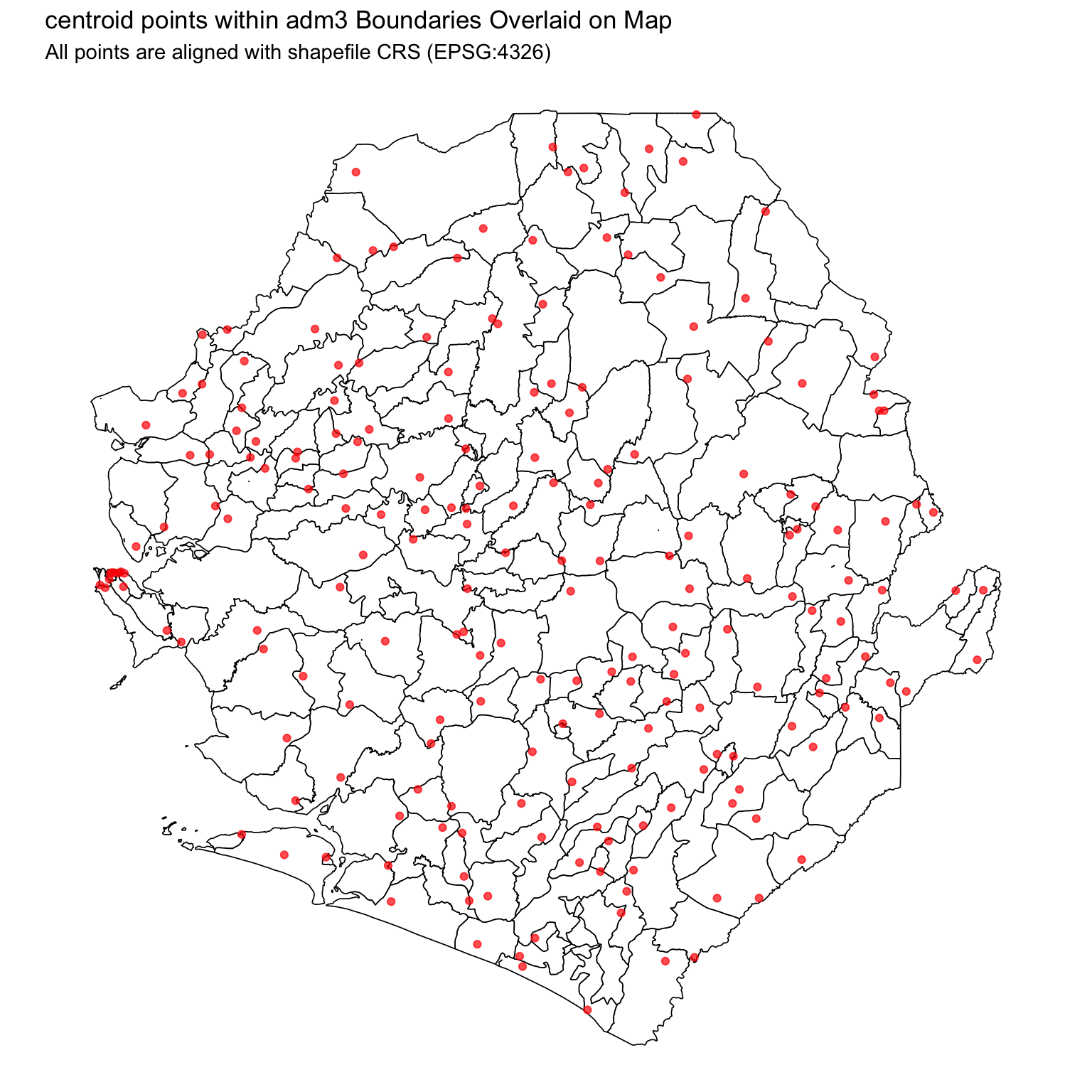
We now shift from name-based matching to coordinate-based joins. When administrative names are missing or unreliable, geographic coordinates provide a robust alternative (that is if they are available). The DHIS2 dataset includes latitude and longitude for health facilities, which allows us to assign records spatially to administrative units in the shapefile. We then calculate the centroid of facilities within each adm3 to later visualize the number of children under 5 confirmed with malaria by adm3.
Step 5.1: Validate and inspect coordinates
Before joining, we need to confirm that the centroids within adm3 boundaries are valid, properly formatted, and fall inside the study area. The checks include:
WarningCoordinate checks
- Ensure latitude and longitude columns exist and contain no missing or zero values.
- Confirm the values are in decimal degrees, not degrees-minutes-seconds or other formats.
- Check that longitudes are in the correct range (e.g., -13 to -10 for Sierra Leone).
- Detect and correct flipped coordinates (e.g., lat/lon accidentally reversed).
- Plot to visually inspect if centroid points fall within the country boundary.
Check Missing Coordinates
Let’s begin by checking for any missing latitude or longitude values in the dataset. These must be addressed before proceeding with coordinate-based joins.
To adapt the code:
- Lines 2 and 3: Replace
dhis2_dfwith your dataset name, and updatelatandlonif your coordinate columns have different names.
To adapt the code:
- Lines 2 and 3: Replace
dhis2_dfwith your dataset name, and updatelatandlonif your coordinate columns have different names.
Looks like there are no missing coordinates. However, if some records are missing coordinates, we can flag these for review and manual inspection.
Check if Coordinates in Decimal Degrees
Most spatial joins require coordinates in decimal degrees such as 7.7675. But some records may use Degree-Minute-Second format such as 7°46′3.93″N, which will cause errors.
Before proceeding, we check for DMS patterns using a simple detection function.
Show the code
# function to detect DMS format using common symbols for
# degrees, minutes, or seconds
detect_dms <- function(x) {
grepl("[°º].*['′\"″]", x)
}
# filter rows where lat or lon appears to be in DMS format
dms_detected <- dhis2_df |>
dplyr::filter(detect_dms(lat) | detect_dms(lon)) |>
dplyr::distinct(adm1, adm2, adm3, lat, lon)
# print summary
cli::cli_h2("DMS Coordinate Check")
cli::cli_alert_info(
"Number of rows with suspected DMS format: {nrow(dms_detected)}"
)
cat("\n")
dms_detectedTo adapt the code:
- Line 7: Replace
dhis2_dfwith your dataset name. - Lines 8 and 9: Update
latandlonif your coordinate columns have different names. - Line 9: Adjust
adm1,adm2,adm3to match your relevant identifier columns for context.
Show the code
# filter rows where lat or lon appears to be in DMS format
dms_detected = (
dhis2_df.loc[
dhis2_df["lat"].apply(detect_dms_value)
| dhis2_df["lon"].apply(detect_dms_value),
["adm1", "adm2", "adm3", "lat", "lon"]
]
.drop_duplicates()
)
cli_header("DMS Coordinate Check")
cli_info(f"Number of rows with suspected DMS format: {len(dms_detected)}")
print(dms_detected)To adapt the code:
- Line 3: Replace
dhis2_dfwith your dataset name. - Lines 4 and 5: Update
latandlonif your coordinate columns have different names. - Line 6: Adjust
adm1,adm2,adm3to match your relevant identifier columns for context.
Only 3 rows were flagged as using DMS formatting. These entries include units from KONO, PUJEHUN and TONKOLILI, suggesting that most of the dataset already uses decimal degrees. The flagged records will be converted to decimal format in the next step.
Show the code
# check if DMS values were successfully converted
check_output <- dhis2_df |>
dplyr::filter(detect_dms(lat) | detect_dms(lon)) |>
dplyr::distinct(adm1, adm2, adm3, lat, lon) |>
dplyr::mutate(
lat_fixed = parzer::parse_lat(lat),
lon_fixed = parzer::parse_lon(lon)
)
# apply conversion to full dataset
dhis2_df_clean <- dhis2_df |>
dplyr::mutate(
lat = parzer::parse_lat(lat),
lon = parzer::parse_lon(lon)
)
# print summary of conversion
cli::cli_h2("DMS Coordinate Conversion Summary")
check_outputTo adapt the code:
- Lines 2 and 11: Replace
dhis2_dfwith your dataset name. - Lines 2–7 and 12–14: Update
latandlonif your coordinate columns have different names.
Show the code
# check if DMS values were successfully converted
check_output = (
dhis2_df.loc[
dhis2_df["lat"].apply(detect_dms_value)
| dhis2_df["lon"].apply(detect_dms_value),
["adm1", "adm2", "adm3", "lat", "lon"]
]
.drop_duplicates()
.assign(
lat_fixed=lambda x: x["lat"].apply(parse_coord),
lon_fixed=lambda x: x["lon"].apply(parse_coord),
)
)
# apply conversion to full dataset
dhis2_df_clean = dhis2_df.copy()
dhis2_df_clean["lat"] = dhis2_df_clean["lat"].apply(parse_coord)
dhis2_df_clean["lon"] = dhis2_df_clean["lon"].apply(parse_coord)
cli_header("DMS Coordinate Conversion Summary")
check_outputTo adapt the code:
- Lines 2 and 17: Replace
dhis2_dfwith your dataset name. - Lines 4–5 and 18–19: Update
latandlonif your coordinate columns have different names.
The lat_fixed and lon_fixed columns confirm that our DMS-formatted coordinates were accurately parsed into decimal degrees. These cleaned values are now stored in dhis2_df_clean.
Check if Coordinates are Flipped
Sometimes, latitude and longitude values are accidentally swapped. For example, a latitude of -12.345 and a longitude of 8.765 when it should be the other way around. This can place points in the wrong hemisphere or completely outside the country of interest. In this sub-section we run a basic check to flag potentially flipped coordinates.
TipHow we detect flipped coordinates
When datasets contain geographic coordinates, a common error is accidentally swapping latitude and longitude values. This can cause points to appear in the wrong country or even on the wrong continent.
To detect possible flipped coordinates, we use a bounding box approach:
- Extract the geographic bounding box from the shapefile, which gives the valid range of latitudes and longitudes for the country.
- For each row in the dataset:
- Check if the latitude falls within the longitude range of the bounding box.
- Check if the longitude falls within the latitude range.
- If both conditions are met, it suggests the values may have been flipped.
This method uses spatial boundaries rather than summary statistics, making it more robust across countries with wide geographic spreads (e.g., Nigeria, DRC).
Show the code
# get bounding box from the shapefile
bbox <- sf::st_bbox(shp_adm3)
# create `possibly_flipped` column in the main dataset
dhis2_df_flagged <- dhis2_df_clean |>
dplyr::mutate(
out_of_bounds = lat < bbox[['ymin']] |
lat > bbox[['ymax']] |
lon < bbox[['xmin']] |
lon > bbox[['xmax']],
looks_flipped = lat > bbox[['xmin']] &
# lat in lon range
lat < bbox[['xmax']] &
lon > bbox[['ymin']] &
# lon in lat range
lon < bbox[['ymax']],
possibly_flipped = looks_flipped
)
# quick summary output
cli::cli_h2("Bounding Box Coordinate Check")
cli::cli_alert_info(
"Out-of-bounds rows: {sum(dhis2_df_flagged$out_of_bounds)}"
)
cli::cli_alert_info(
"Possible flipped rows: {sum(dhis2_df_flagged$possibly_flipped)}"
)
# check output
dhis2_df_flagged |>
dplyr::filter(possibly_flipped) |>
dplyr::select(adm0, adm1, adm2, adm3, lon, lat)To adapt the code:
- Lines 2 and 5: Replace
dhis2_df_cleanwith your dataset name andshp_adm3with your shapefile name if different. - Lines 6–13: Update
latandlonif your coordinate columns have different names. - Line 32: Adjust
adm0,adm1,adm2,adm3to match your relevant identifier columns for context. - It works well when latitudes and longitudes fall in clearly separated ranges (e.g., lat ~8, lon ~–11 in Sierra Leone).
- ⚠️ In countries like Nigeria, where both lat and lon values can fall in similar ranges (e.g., 11°N, 11°E), this check may produce false positives. Use with caution and review flagged rows manually.
Show the code
# get bounding box from the shapefile
xmin, ymin, xmax, ymax = shp_adm3.total_bounds
# create flags in the main dataset
dhis2_df_flagged = dhis2_df_clean.copy()
dhis2_df_flagged["out_of_bounds"] = (
(dhis2_df_flagged["lat"] < ymin)
| (dhis2_df_flagged["lat"] > ymax)
| (dhis2_df_flagged["lon"] < xmin)
| (dhis2_df_flagged["lon"] > xmax)
)
dhis2_df_flagged["possibly_flipped"] = (
(dhis2_df_flagged["lat"] > xmin)
& (dhis2_df_flagged["lat"] < xmax)
& (dhis2_df_flagged["lon"] > ymin)
& (dhis2_df_flagged["lon"] < ymax)
)
cli_header("Bounding Box Coordinate Check")
cli_info(f"Out-of-bounds rows: {dhis2_df_flagged['out_of_bounds'].sum()}")
cli_info(f"Possible flipped rows: {dhis2_df_flagged['possibly_flipped'].sum()}")
dhis2_df_flagged.loc[
dhis2_df_flagged["possibly_flipped"],
["adm0", "adm1", "adm2", "adm3", "lon", "lat"]
]To adapt the code:
- Lines 2 and 5: Replace
dhis2_df_cleanwith your dataset name andshp_adm3with your shapefile name if different. - Lines 6–13: Update
latandlonif your coordinate columns have different names. - Line 25: Adjust
adm0,adm1,adm2,adm3to match your relevant identifier columns for context. - This check works best when latitude and longitude ranges are clearly separated. Review flagged rows manually in countries where ranges overlap.
These results include three rows with coordinates that either fall outside the expected bounding box or appear to be flipped (For example, cases where latitude is negative or outside the plausible range). Since Sierra Leone has negative longitudes but not latitudes, such records should be flagged for review or corrected manually based on contextual program knowledge.
Now we will convert this cleaned dataset into an sf object and begin spatially joining each row to its corresponding administrative unit based on location.
Show the code
# reverse flipped coordinates
dhis2_df_corrected <- dhis2_df_flagged |>
dplyr::mutate(
lat_temp = dplyr::if_else(possibly_flipped, lon, lat),
lon_temp = dplyr::if_else(possibly_flipped, lat, lon),
lat = lat_temp,
lon = lon_temp
) |>
dplyr::select(-lat_temp, -lon_temp)
# check output
dhis2_df_corrected |>
dplyr::filter(possibly_flipped) |>
dplyr::select(adm0, adm1, adm2, adm3, lon, lat)To adapt the code:
- Lines 2 and 3–7: Update variable names if your dataset or coordinate columns have different names.
- Line 14: Adjust
adm0,adm1,adm2,adm3to match your relevant identifier columns for context.
Show the code
# reverse flipped coordinates
dhis2_df_corrected = dhis2_df_flagged.copy()
lat_temp = np.where(
dhis2_df_corrected["possibly_flipped"],
dhis2_df_corrected["lon"],
dhis2_df_corrected["lat"],
)
lon_temp = np.where(
dhis2_df_corrected["possibly_flipped"],
dhis2_df_corrected["lat"],
dhis2_df_corrected["lon"],
)
dhis2_df_corrected["lat"] = lat_temp
dhis2_df_corrected["lon"] = lon_temp
dhis2_df_corrected.loc[
dhis2_df_corrected["possibly_flipped"],
["adm0", "adm1", "adm2", "adm3", "lon", "lat"]
]To adapt the code:
- Lines 2 and 3–15: Update variable names if your dataset or coordinate columns have different names.
- Line 19: Adjust
adm0,adm1,adm2,adm3to match your relevant identifier columns for context.
Step 5.2: Check and align coordinate reference system (CRS)
Before performing any spatial join, it’s essential to ensure that the DHIS2 data and the shapefile use the same coordinate reference system. Most shapefiles are in geographic coordinates using EPSG:4326, but your DHIS2 data may not be explicitly tagged.
We’ll check the CRS of both datasets and, if needed, set or transform the CRS of the DHIS2 data to match the shapefile.
Show the code
# check CRS of shapefile
shp_crs <- sf::st_crs(shp_adm3)
# convert DHIS2 data to an sf object
dhis2_df_sf <- dhis2_df_corrected |>
# only keep rows with valid coordinates
dplyr::filter(!is.na(lat), !is.na(lon)) |>
# assume input is EPSG:4326
sf::st_as_sf(coords = c("lon", "lat"), crs = 4326, remove = FALSE)
# reproject if CRS mismatch
if (sf::st_crs(dhis2_df_sf) != shp_crs) {
dhis2_df_sf <- sf::st_transform(dhis2_df_sf, shp_crs)
}
# summary
cli::cli_h2("CRS Alignment Summary")
cli::cli_alert_info("Shapefile CRS: {.strong {shp_crs$input}}")
cli::cli_alert_info(
"Intervention data CRS: {.strong {sf::st_crs(dhis2_df_sf)$input}}")
crs_summary <- data.frame(
dataset = c("Shapefile", "DHIS2 point data"),
crs = c(shp_crs$input, sf::st_crs(dhis2_df_sf)$input)
)
crs_summaryTo adapt the code:
- Line 2: Replace
shp_adm3with the name of your own shapefile object. - Lines 5 and 6: Ensure your dataset (
dhis2_df_corrected) contains numericlatandloncolumns before converting tosfobject. - Line 8: If your coordinates use a different input CRS (e.g., not
EPSG:4326), update thecrs = 4326argument accordingly. - Note: In this demonstration, coordinates represent centroid points within
adm3boundaries.
Show the code
# check CRS of shapefile and assign a fallback if missing
if shp_adm3.crs is None:
shp_adm3 = shp_adm3.set_crs("EPSG:4326")
shp_crs = shp_adm3.crs
# convert DHIS2 data to a GeoDataFrame
dhis2_df_sf = gpd.GeoDataFrame(
dhis2_df_corrected.dropna(subset=["lat", "lon"]),
geometry=gpd.points_from_xy(
dhis2_df_corrected.dropna(subset=["lat", "lon"])["lon"],
dhis2_df_corrected.dropna(subset=["lat", "lon"])["lat"],
),
crs="EPSG:4326",
)
# reproject if CRS mismatch
if dhis2_df_sf.crs != shp_crs:
dhis2_df_sf = dhis2_df_sf.to_crs(shp_crs)
cli_header("CRS Alignment Summary")
cli_info(f"Shapefile CRS: {shp_crs}")
cli_info(f"Intervention data CRS: {dhis2_df_sf.crs}")
crs_summary = pd.DataFrame({
"dataset": ["Shapefile", "DHIS2 point data"],
"crs": [str(shp_crs), str(dhis2_df_sf.crs)],
})
crs_summaryTo adapt the code:
- Lines 2–4: Replace
shp_adm3with the name of your own shapefile object. The fallbackset_crs("EPSG:4326")ensures the shapefile has a CRS assigned before reprojection. - Lines 7–14: Ensure your dataset (
dhis2_df_corrected) contains numericlatandloncolumns before converting to a GeoDataFrame. - Line 13: If your coordinates use a different input CRS, update
crs="EPSG:4326"accordingly.
Both the shapefile and DHIS2 dataset are using the same CRS (EPSG:4326). We’ve also successfully converted the DHIS2 data with centroid points within adm3 boundaries into a point-based spatial layer.
This means we can now confidently overlay the centroid points on top of the administrative boundaries and proceed with spatial joins.
Let us plot both of these together now.
Show the code
# plot shapefile and points
ggplot2::ggplot() +
ggplot2::geom_sf(
data = shp_adm3,
fill = "white",
color = "black",
size = 0.3
) +
ggplot2::geom_sf(data = dhis2_df_sf, color = "red", size = 1.5, alpha = 0.7) +
ggplot2::labs(
title = "centroid points within adm3 Boundaries Overlaid on Map",
subtitle = "All points are aligned with shapefile CRS (EPSG:4326)"
) +
ggplot2::theme_void()
NoteOutput
To adapt the code:
- Line 3: Replace
shp_adm3with your own shapefile if using a different admin level or region. - Line 8: Ensure
dhis2_df_sfis your dataset with coordinates converted to ansfobject with the correct CRS. - Lines 3–7 and 8: Adjust the
fill,color, andsizeoptions ingeom_sf()as needed to match your visualization style or presentation needs. - Lines 9–11: Update the plot title and subtitle to reflect your dataset and context.
Show the code
fig, ax = plt.subplots(figsize=(8, 8))
# set the aspect once on the axes; pass aspect=None to gdf.plot() so
# geopandas does not recompute an aspect from each layer's bounds (which
# can yield non-finite values when a layer has empty or degenerate
# geometry and trigger `aspect must be finite and positive`)
ax.set_aspect("equal")
shp_adm3.plot(
ax=ax, facecolor="white", edgecolor="black", linewidth=0.3, aspect=None
)
dhis2_df_sf.plot(
ax=ax, color="red", markersize=12, alpha=0.7, aspect=None
)
ax.set_title(
"centroid points within adm3 Boundaries Overlaid on Map\n"
"All points are aligned with shapefile CRS (EPSG:4326)"
)
ax.set_axis_off()
plt.show()
NoteOutput
To adapt the code:
- Line 2: Replace
shp_adm3with your own shapefile if using a different admin level or region. - Line 3: Ensure
dhis2_df_sfis your dataset with coordinates converted to a GeoDataFrame with the correct CRS. - Lines 2–3: Adjust the fill, colour, and marker size options as needed.
- Lines 4–7: Update the plot title and subtitle to reflect your dataset and context.
We have successfully cleaned and aligned our coordinate data. The centroid points within adm3 boundaries now correctly overlay the shapefile, and we’re ready for the next step: spatially joining these points to admin units.
Step 5.3: Aggregate coordinates to the adm3 level
After validating and parsing facility coordinates, before joining them to the shapefile, the next step is to aggregate them to the adm3 level. This involves calculating a representative centroid for each adm3 by averaging the latitude and longitude of facilities within its boundary. These centroids provide a spatial reference point for visualizing aggregated indicators.
We then join these aggregated centroids with DHIS2 indicators for 2023, which are grouped and summed at the adm3 level. The result is a dataset where each administrative unit is linked to both its aggregated malaria indicators and its corresponding centroid coordinate, ready for mapping and further analysis.
Show the code
# get the hf centroids at the adm3 level
dhis2_hf_coords <- dhis2_df_sf |>
sf::st_drop_geometry() |>
dplyr::select(adm0, adm1, adm2, adm3, lat, lon) |>
dplyr::group_by(adm0, adm1, adm2, adm3) |>
dplyr::summarise(
lon = mean(lon, na.rm = T),
lat = mean(lat, na.rm = T),
.groups = "drop"
)
# get indicators for 2023 at the adm3 level and join back
dhis2_df_sf <- dhis2_df_sf |>
sf::st_drop_geometry() |>
dplyr::select(
adm0,
adm1,
adm2,
adm3,
year,
conf_u5
) |>
dplyr::filter(year == 2023) |>
dplyr::group_by(adm0, adm1, adm2, adm3, year) |>
dplyr::summarise(
conf_u5 = sum(conf_u5, na.rm = TRUE),
.groups = "drop"
) |>
# join the coords
dplyr::left_join(
dhis2_hf_coords,
by = c("adm0", "adm1", "adm2", "adm3")
) |>
sf::st_as_sf(coords = c("lon", "lat"), crs = sf::st_crs(shp_adm3), remove = FALSE)To adapt the code:
- Lines 2 and 3–4: Adjust the selected columns to match your dataset (e.g., adm levels, lat/lon field names, or any additional grouping variables).
- Lines 14 and 17: Replace the indicator variables (
year,conf_u5) with the indicators available in your dataset. - Line 22: Update the join keys (
adm0–adm3) if your dataset uses different administrative levels.
Show the code
# get the centroid coordinates at the adm3 level
dhis2_hf_coords = (
pd.DataFrame(dhis2_df_sf.drop(columns="geometry"))
.groupby(["adm0", "adm1", "adm2", "adm3"], as_index=False)
.agg(lon=("lon", "mean"), lat=("lat", "mean"))
)
# get indicators for 2023 at adm3 level and join back coordinates
dhis2_df_sf = (
pd.DataFrame(dhis2_df_sf.drop(columns="geometry"))
[["adm0", "adm1", "adm2", "adm3", "year", "conf_u5"]]
.loc[lambda x: x["year"].astype(str) == "2023"]
.groupby(["adm0", "adm1", "adm2", "adm3", "year"], as_index=False)
.agg(conf_u5=("conf_u5", "sum"))
.merge(dhis2_hf_coords, on=["adm0", "adm1", "adm2", "adm3"], how="left")
)
dhis2_df_sf = gpd.GeoDataFrame(
dhis2_df_sf,
geometry=gpd.points_from_xy(dhis2_df_sf["lon"], dhis2_df_sf["lat"]),
crs=shp_adm3.crs,
)To adapt the code:
- Lines 4 and 5: Adjust the selected columns to match your dataset.
- Lines 12 and 15: Replace
yearandconf_u5with the indicators available in your dataset. - Line 17: Update the join keys (
adm0–adm3) if your dataset uses different administrative levels.
Step 5.4: Spatial join of centroid points to shapefile
After preparing and validating our coordinate data, we’re now ready to join our DHIS2 dataset with centroid points within adm3 boundaries to administrative boundaries using a spatial join. This step assigns each centroid point to its corresponding polygon such as district or chiefdom, allowing us to summarize and analyze testing coverage by geographic area.
R provides several methods for determining how points relate to polygons during spatial joins::
sf::st_contains: Points contained within polygon (most common method, used in the code below)sf::st_intersects: Point touches or is within polygonsf::st_within: Point is completely within polygon (inverse of contains)sf::st_nearest_feature: Assigns to closest polygon when boundaries are ambiguous
Show the code
# joined to shapefile using spatial coordinates
dhis2_df_spatial_join <- sf::st_join(
dplyr::select(shp_adm3, geometry),
dhis2_df_sf,
join = sf::st_contains
) |>
dplyr::distinct(.keep_all = TRUE)
# check for unmatched rows
unmatched_points <- dhis2_df_spatial_join |> dplyr::filter(is.na(adm3))
cli::cli_h2("Spatial Join Validation")
cli::cli_alert_info("Number of unmatched points: {nrow(unmatched_points)}")
# check output
head(dhis2_df_spatial_join)To adapt the code:
- Lines 2 and 3: Replace
shp_adm3with your polygon shapefile anddhis2_df_sfwith your point-based data (must be an sf object). - Line 6: Adjust the final
dplyr::distinct()to retain the relevant administrative levels and variables of interest (e.g.,conf_u5) and drop any duplicates. - Line 9: Adjust
adm3to match your relevant identifier column for checking unmatched points. - Important: The order of datasets in
sf::st_join()determines both the output geometry and which spatial predicate to use:- If we want the polygon geometry in results → mention polygons first:
sf::st_join(polygons, points, join = sf::st_contains). - If we want the point geometry in results → mention points first:
sf::st_join(points, polygons, join = sf::st_within). - We want to join our shapefile to our tabular data, so we mention
shp_adm3first.
- If we want the polygon geometry in results → mention polygons first:
sf::st_containsandsf::st_withinare inverse relationships - a polygon contains a point if and only if the point is within the polygon.
Python provides the same spatial predicates through geopandas.sjoin():
predicate="contains": polygons contain points.predicate="intersects": polygons touch or contain points.predicate="within": points are within polygons, usually with points as the left dataset.sjoin_nearest(): assigns the nearest polygon when boundaries are ambiguous.
Show the code
# join to shapefile using spatial coordinates
dhis2_df_spatial_join = (
gpd.sjoin(
shp_adm3[["geometry"]],
dhis2_df_sf,
how="left",
predicate="contains"
)
.drop(columns="index_right", errors="ignore")
.drop_duplicates(subset=["adm0", "adm1", "adm2", "adm3", "year", "conf_u5"])
)
# check for unmatched rows
unmatched_points = dhis2_df_spatial_join.loc[dhis2_df_spatial_join["adm3"].isna()]
cli_header("Spatial Join Validation")
cli_info(f"Number of unmatched points: {len(unmatched_points)}")
dhis2_df_spatial_join.head()To adapt the code:
- Lines 4 and 5: Replace
shp_adm3with your polygon shapefile anddhis2_df_sfwith your point-based data. - Line 12: Adjust the final duplicate subset to retain the relevant administrative levels and variables of interest.
- Line 16: Adjust
adm3to match your relevant identifier column for checking unmatched points. - If you want point geometry in the output, place
dhis2_df_sfon the left and usepredicate="within".
We have successfully joined the DHIS2 data to the shapefile. All centroid points within adm3 boundaries now inherit administrative context (e.g., district, chiefdom) based on where they fall within the shapefile polygons.
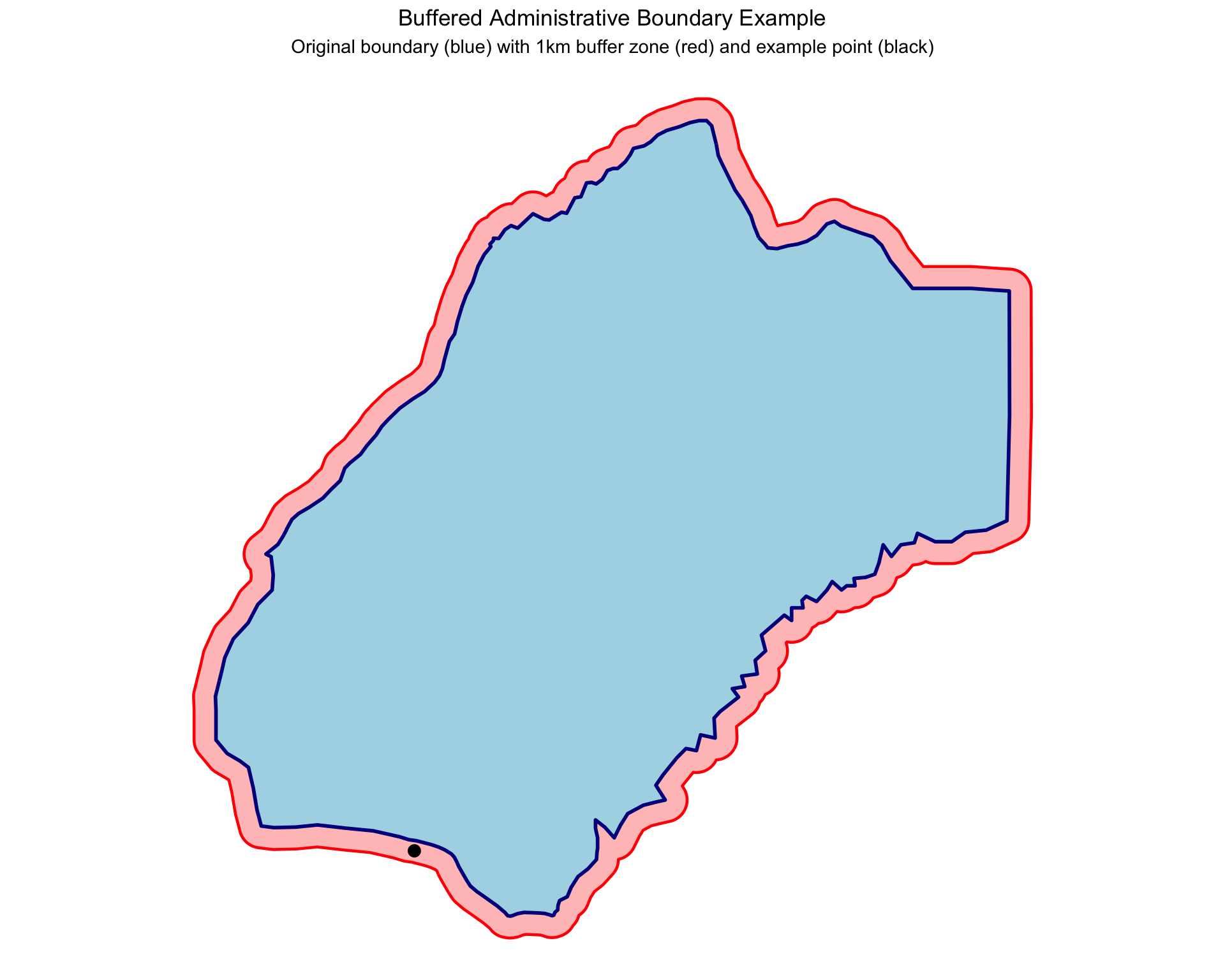
Step 5.5: Using buffered joins for near-miss points (Alternative step 5.4)
Sometimes coordinate-based joins fail because points fall just outside administrative boundaries due to GPS errors, boundary digitization differences, or coordinate rounding. In these cases, a buffered join can help by creating a small tolerance zone around boundaries.
It is important to note that this step is an alternative to Step 5.3, and should not be done in addition to the standard spatial join.
WarningPoints outside boundaries
Consider buffered joins when:
- Points fall just outside boundaries (especially near borders)
- GPS coordinates from mobile devices (lower accuracy): buffer 500m - 1km
- Historical data (boundaries may have changed): buffer 1km - 3km
- Health facilities near administrative borders: buffer 500m - 2km
- Survey clusters (displaced for privacy DHS for example): buffer 100m - 500m
Note: These are suggested buffer distances - adjust based on your specific data quality and context.
While buffering recovers near-miss points, it can also:
- Assign points to incorrect administrative units in dense boundary areas
- Create overlapping claims between adjacent units
- Mask genuine data quality issues that should be addressed at source
Buffer decisions should be determined by understanding of context as well as data integrity. Always assess whether unmatched points are genuinely close to boundaries (GPS precision issues) or far away (data quality problems) before applying buffers.
In this section we will create a buffered version of shp_adm3 called shp_adm3_buffered, and then show an example of a coordinate that falls outside MALEMA but should be assigned to MALEMA chiefdom through buffering.
To adapt the code:
- Line 5: Adjust
dist = 1000to change buffer size (in meters). Use different buffer distances for different administrative levels if needed. - Line 6: Replace
crs = 4326with output ofsf::st_crs(shp_adm3)to preserve original CRS.- Line 4: Note: We transform to
crs = 3857(Web Mercator) for accurate meter-based buffering.
- Line 4: Note: We transform to
To adapt the code:
- Line 4: Adjust
.buffer(1000)to change buffer size in meters. - Line 5: Replace
epsg=4326withshp_adm3.crsto preserve the original CRS. - Line 3: The code transforms to EPSG:3857 for meter-based buffering.
Now let’s create an example coordinate that falls just outside MALEMA chiefdom but should logically belong to it:
Show the code
# select MALEMA chiefdom for our example
malema_original <- shp_adm3 |>
dplyr::filter(adm3 == "MALEMA")
malema_buffered <- shp_adm3_buffered |>
dplyr::filter(adm3 == "MALEMA")
# create example point that falls just outside MALEMA but within
# buffer zone (this simulates a GPS point with slight inaccuracy)
example_point <- data.frame(
# 10.85 W (negative for west)
lon = -10.85,
# 7.641 N (positive for north)
lat = 7.641
) |>
sf::st_as_sf(coords = c("lon", "lat"), crs = 4326)
# create visualization
ggplot2::ggplot() +
# plot the buffer first (so it appears behind)
ggplot2::geom_sf(
data = malema_buffered,
fill = "red",
alpha = 0.3,
color = "red",
size = 0.8
) +
# plot the original boundary on top
ggplot2::geom_sf(
data = malema_original,
fill = "lightblue",
color = "darkblue",
size = 1
) +
# add the example point
ggplot2::geom_sf(
data = example_point,
color = "black",
size = 3,
# filled circle
shape = 19
) +
ggplot2::labs(
title = "Buffered Administrative Boundary Example",
subtitle = "Original boundary (blue) with 1km buffer zone (red) and example point (black)"
) +
ggplot2::theme_void() +
ggplot2::theme(
plot.title = ggplot2::element_text(hjust = 0.5),
plot.subtitle = ggplot2::element_text(hjust = 0.5)
)
NoteOutput
Show the code
# select MALEMA chiefdom for the example
malema_original = shp_adm3.loc[shp_adm3["adm3"] == "MALEMA"]
malema_buffered = shp_adm3_buffered.loc[shp_adm3_buffered["adm3"] == "MALEMA"]
# create example point that falls just outside MALEMA but within the buffer zone
example_point = gpd.GeoDataFrame(
{"lon": [-10.85], "lat": [7.641]},
geometry=gpd.points_from_xy([-10.85], [7.641]),
crs="EPSG:4326"
)
fig, ax = plt.subplots(figsize=(10, 8))
# set the aspect once on the axes and tell geopandas to skip its own
# aspect computation, which can yield non-finite values for degenerate
# / single-feature layers
ax.set_aspect("equal")
malema_buffered.plot(
ax=ax, color="red", alpha=0.3, edgecolor="red", linewidth=0.8, aspect=None
)
malema_original.plot(
ax=ax, color="lightblue", edgecolor="darkblue", linewidth=1, aspect=None
)
example_point.plot(ax=ax, color="black", markersize=35, aspect=None)
ax.set_title(
"Buffered Administrative Boundary Example\n"
"Original boundary (blue) with 1km buffer zone (red) and example point (black)"
)
ax.set_axis_off()
plt.show()
NoteOutput
The original boundary is shown as the blue fill, but with the 1km buffer (in red) the boundary has changed slightly. Now we can see that the coordinate just outside the border of MALEMA will be included as part of MALEMA chiefdom if shp_adm3_buffered is used. This will be true for any other points in the map that fall within the buffer zones of their nearest administrative units.
If one wished to use the buffered approach to joining their data, they would be looking to use shp_adm3_buffered for their spatial joining instead of shp_adm3.
To adapt the code:
- Lines 2 and 3: Replace
shp_adm3_bufferedwith your polygon shapefile anddhis2_df_sfwith your point-based data (must be an sf object). - Line 6: Adjust the final
dplyr::distinct()to retain the relevant administrative levels and variables of interest (e.g.,conf_u5) and drop any duplicates. - Important: The order of datasets in
sf::st_join()determines both the output geometry and which spatial predicate to use:- If we want the polygon geometry in results → mention polygons first:
sf::st_join(polygons, points, join = sf::st_contains). - If we want the point geometry in results → mention points first:
sf::st_join(points, polygons, join = sf::st_within). - We want to join our shapefile to our tabular data, so we mention
shp_adm3_bufferedfirst.
- If we want the polygon geometry in results → mention polygons first:
sf::st_containsandsf::st_withinare inverse relationships - a polygon contains a point if and only if the point is within the polygon.
To adapt the code:
- Lines 4 and 5: Replace
shp_adm3_bufferedwith your buffered polygon shapefile anddhis2_df_sfwith your point-based data. - Line 11: Adjust the final
.drop_duplicates()to retain the relevant administrative levels and variables of interest. - If you want point geometry in the output, place
dhis2_df_sfon the left and usepredicate="within".
Step 6: Validate both join methods
After successfully demonstrating both attribute-based (name) and coordinate-based joining methods, we need to validate that both approaches produce consistent and complete results. This validation step ensures that our spatial data linkage is robust and that we can confidently use either method depending on data availability and quality.
We’ll compare the results from both join methods to confirm they produce the same spatial coverage and identify any discrepancies that need investigation.
Step 6.1: Prepare both join results for comparison
First, let’s create clean versions of both join results with consistent column names for easy comparison.
Show the code
# name-based join result (from Step 4.5)
name_join_result <- dhis2_df_coord_shp |>
dplyr::mutate(join_method = "Attribute-based Join") |>
as.data.frame() |>
dplyr::select(
adm0,
adm1,
adm2,
adm3,
year,
conf_u5,
join_method
) |>
dplyr::filter(year == 2023) |>
dplyr::group_by(adm0, adm1, adm2, adm3, year, join_method) |>
dplyr::summarise(
conf_u5 = sum(conf_u5, na.rm = TRUE),
.groups = "drop"
) |>
# join back shapefile
dplyr::left_join(
shp_adm3,
by = c("adm0", "adm1", "adm2", "adm3")
)
# coordinate-based join result (from Step 5.3)
coord_join_result <- dhis2_df_spatial_join |>
dplyr::mutate(join_method = "Coordinate-based Join") |>
dplyr::select(
adm0,
adm1,
adm2,
adm3,
conf_u5,
join_method
) |>
# remove unmatched points
dplyr::filter(!is.na(adm3))
# bind both together
joined_plot_data <- dplyr::bind_rows(
name_join_result,
coord_join_result
)
# check summary statistics for conf_u5
joined_plot_data |>
as.data.frame() |>
dplyr::group_by(join_method) |>
dplyr::summarise(
min_conf_u5 = min(conf_u5, na.rm = TRUE),
mean_conf_u5 = mean(conf_u5, na.rm = TRUE),
max_conf_u5 = max(conf_u5, na.rm = TRUE),
n_missing = sum(is.na(conf_u5))
)To adapt the code:
- Lines 10, 16, and 28: Replace
conf_u5with your own malaria indicator. - Lines 5–10 and 23–28: Adjust the selected columns to match your dataset structure and variables of interest.
Show the code
# name-based join result from Step 4.5
name_join_result = (
pd.DataFrame(dhis2_df_coord_shp.drop(columns="geometry"))
.assign(join_method="Attribute-based Join")
[["adm0", "adm1", "adm2", "adm3", "year", "conf_u5", "join_method"]]
# cast year to string so the filter works whether the source column is
# stored as integer or character (R rio import keeps it as character)
.loc[lambda x: x["year"].astype(str) == "2023"]
.groupby(["adm0", "adm1", "adm2", "adm3", "year", "join_method"], as_index=False)
.agg(conf_u5=("conf_u5", "sum"))
.merge(shp_adm3, on=["adm0", "adm1", "adm2", "adm3"], how="left")
)
name_join_result = gpd.GeoDataFrame(name_join_result, geometry="geometry", crs=shp_adm3.crs)
# coordinate-based join result from Step 5.3
coord_join_result = (
dhis2_df_spatial_join
.assign(join_method="Coordinate-based Join")
[["adm0", "adm1", "adm2", "adm3", "conf_u5", "join_method", "geometry"]]
.loc[lambda x: x["adm3"].notna()]
)
# bind both together
joined_plot_data = gpd.GeoDataFrame(
pd.concat([name_join_result, coord_join_result], ignore_index=True, sort=False),
geometry="geometry",
crs=shp_adm3.crs
)
# check summary statistics for conf_u5
joined_plot_data.groupby("join_method").agg(
min_conf_u5=("conf_u5", "min"),
mean_conf_u5=("conf_u5", "mean"),
max_conf_u5=("conf_u5", "max"),
n_missing=("conf_u5", lambda x: x.isna().sum()),
).reset_index()To adapt the code:
- Lines 6, 9 and 18: Replace
conf_u5with your own malaria indicator. - Lines 5–6 and 17–18: Adjust the selected columns to match your dataset structure and variables of interest.
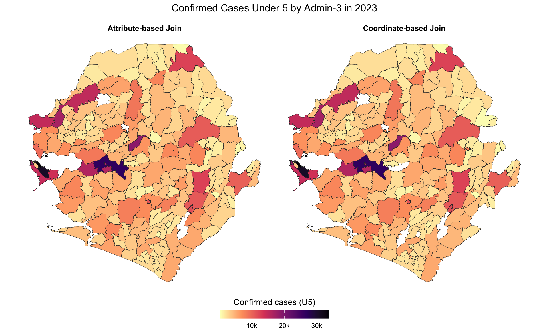
We can see that the join worked as the summary stats for conf_u5 for both datasets are exactly the same.
Step 6.2: Visual validation - side-by-side comparison
Finally, let’s create side-by-side maps to visually confirm that both join methods produce identical spatial patterns. Each polygon in the shapefile should have the same color fill in both maps.
Show the code
adm3_validation_map <- joined_plot_data |>
sf::st_as_sf() |>
ggplot2::ggplot() +
ggplot2::geom_sf(
aes(fill = conf_u5 / 1000),
color = "grey20",
size = 0.15
) +
ggplot2::scale_fill_viridis_c(
option = "A",
direction = -1,
labels = scales::label_number(
accuracy = 1,
# formats as 5k, 10k, 20k
suffix = "k"
),
na.value = "lightgrey",
guide = ggplot2::guide_colorbar(
barwidth = grid::unit(5, "cm"),
barheight = grid::unit(0.4, "cm"),
title.position = "top"
)
) +
ggplot2::facet_wrap(~join_method, nrow = 1) +
ggplot2::labs(
title = "Confirmed Cases Under 5 by Admin-3 in 2023\n",
fill = "Confirmed cases (U5)"
) +
ggplot2::coord_sf(datum = NA) +
ggplot2::theme_void() +
ggplot2::theme(
strip.text = ggplot2::element_text(size = 10, face = "bold"),
legend.position = "bottom",
legend.title = ggplot2::element_text(hjust = 0.5),
plot.title = ggplot2::element_text(hjust = 0.5)
)
# display the plot
adm3_validation_map
# save plot
ggplot2::ggsave(
plot = adm3_validation_map,
here::here("03_output/3a_figures/shapefile_check_conf_adm3.png"),
width = 12,
height = 5,
dpi = 300
)
NoteOutput
To adapt the code:
- Line 5: Replace
conf_u5with your continuous malaria indicator variable. - Lines 25–27: Update plot titles and subtitles to reflect your specific context.
Show the code
NoteOutput
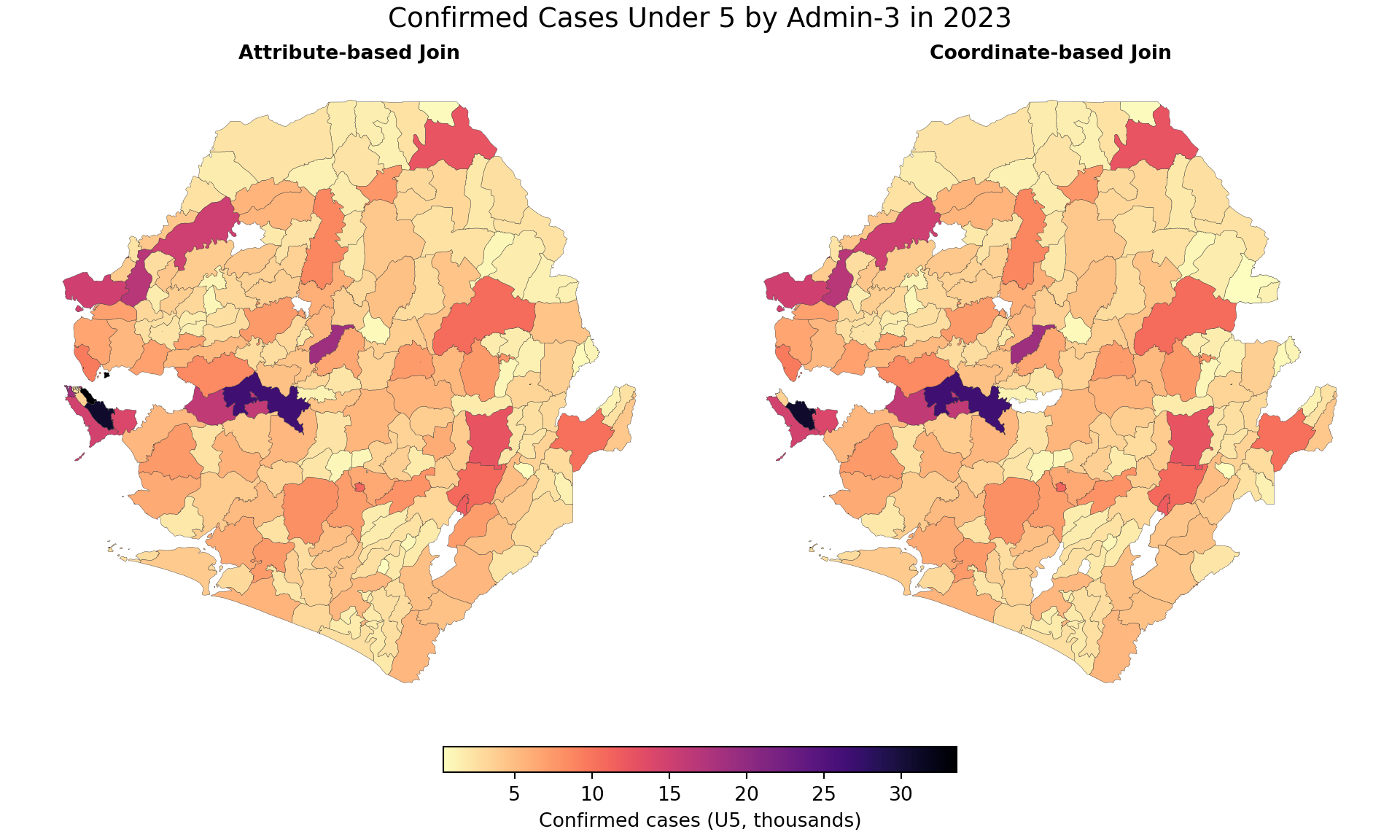
To adapt the code:
- Line 4: Replace
conf_u5with your continuous malaria indicator variable. - Line 6: Update the plot title to reflect your specific context.
All 208 areas joined successfully with identical testing rates. The side-by-side maps confirm everything aligned correctly. Do use visual inspections such as this to see whether your merge worked properly and catch any potential data issues early.
Step 7: Save data
In this step we save the final merged DHIS2 data with our shapefile.
There are a number of formats available for saving your data, all of which have been demonstrated in Step 7 of the Shapefile Management and Customization page. In this example, we will use the simple RDS format, ensuring that in future use when we load it we convert it to an sf object:
Show the code
To adapt the code:
- Lines 2–4 and 7–9: Be sure to adapt the file paths and objects for files to be saved appropriately before saving.
Show the code
save_path = Path(surv_path) / "processed"
save_path.mkdir(parents=True, exist_ok=True)
# save the name-based joined data
dhis2_df_coord_shp.to_file(
save_path / "sle_dhis2_df_name_joined_adm3.gpkg",
layer="name_joined_adm3",
driver="GPKG"
)
# save the coordinate-based joined data
dhis2_df_spatial_join.to_file(
save_path / "sle_dhis2_df_coord_joined_adm3.gpkg",
layer="coord_joined_adm3",
driver="GPKG"
)To adapt the code:
- Lines 2–4 and 10–12: Adapt the file paths and objects before saving.
- Use GeoPackage for spatial outputs and CSV or Parquet for non-spatial tables.
Summary
In this section, we walked through the full preparation of coordinate data for spatial analysis. We identified and converted DMS-formatted values, flagged and corrected possible flipped coordinates using both bounding box logic and visual checks, and ensured both datasets shared a consistent CRS. After converting the DHIS2 data to an sf object, we successfully performed a spatial join with the shapefile and visualized the results using clean, categorized maps. This section serves as a key reference for anyone preparing point-based datasets for integration with administrative boundaries, return to it anytime you need to align and validate geospatial data.
Full code
Find the full code script for merging shapefiles with tabular data below.
Show full code
################################################################################
############## ~ Merging shapefiles with tabular data full code ~ ##############
################################################################################
### Step 1: Install and load packages ------------------------------------------
# Check if 'pacman' is installed; install it if missing
if (!requireNamespace("pacman", quietly = TRUE)) {
install.packages("pacman")
}
# Load all required packages using pacman
pacman::p_load(
sf, # for reading and handling shapefiles
rio, # for importing Excel files (replaces readxl)
dplyr, # for data manipulation
stringr, # for string cleaning and formatting
ggplot2, # for creating plots
cli, # for styled console output
here # for cross-platform file paths
)
# sntutils has a number of useful helper functions for data
# management and cleaning
if (!requireNamespace("sntutils", quietly = TRUE)) {
devtools::install_github("ahadi-analytics/sntutils")
}
# for parsing coordinates
if (!requireNamespace("parzer", quietly = TRUE)) {
remotes::install_github("ropensci/parzer")
}
### Step 2: Import and examine data --------------------------------------------
# import shapefile
shp_adm3 <- readRDS(
here::here(
"1.1_foundational",
"1.1a_administrative_boundaries",
"processed",
"sle_spatial_adm3_2021.rds"
)
) |>
# ensure output remains a valid sf object for downstream joins
sf::st_as_sf()
# surv data path
surv_path <- here::here("1.2_epidemiology", "1.2a_routine_surveillance")
# get malaria
dhis2_df <- rio::import(
here::here(
surv_path,
"raw",
"clean_malaria_routine_data_final.rds"
)
)
# check DHIS2 data and shapefile
cli::cli_h2("DHIS2 data")
dhis2_df |>
dplyr::distinct(adm0, adm1, adm2, adm3) |>
dplyr::arrange(adm0, adm1, adm2, adm3) |>
head(n = 10)
cli::cli_h2("Adm3 shapefile")
shp_adm3 |>
dplyr::distinct(adm0, adm1, adm2, adm3) |>
dplyr::arrange(adm0, adm1, adm2, adm3) |>
head(n = 10)
### Step 3: Identify and fix hierarchy mismatches ------------------------------
# initial cleaning
dhis2_df <- dhis2_df |>
dplyr::mutate(
adm0 = toupper(adm0),
adm2 = toupper(adm1),
adm3 = toupper(adm3),
adm2 = stringr::str_replace(
adm2,
stringr::fixed(" DISTRICT"),
""
),
adm3 = stringr::str_replace(
adm3,
stringr::fixed(" CHIEFDOM"),
""
)
) |>
dplyr::mutate(
adm1 = dplyr::case_when(
adm2 %in% c("KAILAHUN", "KENEMA", "KONO") ~
"EASTERN",
adm2 %in% c("BOMBALI", "FALABA", "KOINADUGU", "TONKOLILI") ~
"NORTH EAST",
adm2 %in% c("KAMBIA", "KARENE", "PORT LOKO") ~
"NORTH WEST",
adm2 %in% c("BO", "BONTHE", "MOYAMBA", "PUJEHUN") ~
"SOUTHERN",
adm2 %in% c("WESTERN AREA RURAL", "WESTERN AREA URBAN") ~
"WESTERN"
)
)
# check DHIS2 data and shapefile
cli::cli_h2("DHIS2 data (initial cleaning) ")
dhis2_df |>
dplyr::distinct(adm0, adm1, adm2, adm3) |>
dplyr::arrange(adm0, adm1, adm2, adm3) |>
head(n = 10)
cli::cli_h2("Adm3 shapefile")
shp_adm3 |>
dplyr::distinct(adm0, adm1, adm2, adm3) |>
dplyr::arrange(adm0, adm1, adm2, adm3) |>
head(n = 10)
### Step 4: Join by Administrative Names (Attribute Joins) ---------------------
#### Step 4.1: Assessing whether the two datasets can join ---------------------
# get distinct admin names from dhis2
dhis2_admins <-
dhis2_df |>
dplyr::distinct(adm0, adm1, adm2, adm3)
# drop geometry for name-only joins
shp_names <-
shp_adm3 |>
sf::st_drop_geometry() |>
dplyr::distinct(adm0, adm1, adm2, adm3)
# inner join to count matches (polygons ∩ dhis2)
shp_with_dhis2 <-
shp_names |>
dplyr::inner_join(
dhis2_admins,
by = c("adm0", "adm1", "adm2", "adm3")
)
# polygons with no matching dhis2 admin (shapefile ▷ dhis2)
polygons_without_dhis2 <-
shp_names |>
dplyr::anti_join(
dhis2_admins,
by = c("adm0", "adm1", "adm2", "adm3")
)
# dhis2 admins with no matching polygon (dhis2 ▷ shapefile)
dhis2_without_polygons <-
dhis2_admins |>
dplyr::anti_join(
shp_names,
by = c("adm0", "adm1", "adm2", "adm3")
)
# counts for clear diagnostics
total_polygons <- nrow(shp_adm3)
matched_polygons <- nrow(shp_with_dhis2)
polygons_no_match <- nrow(polygons_without_dhis2)
dhis2_no_match <- nrow(dhis2_without_polygons)
# report
cli::cli_h2("Admin join diagnostics (adm0 to adm3)")
# polygons perspective
cli::cli_alert_success(
"Shapefile admin units (unique): {total_polygons}"
)
cli::cli_alert_success(
"Matched with DHIS2: {matched_polygons}"
)
# DHIS2 perspective
cli::cli_alert_warning(
"Unmatched DHIS2 admin units (no polygon): {dhis2_no_match}"
)
cli::cli_alert_warning(
"Unmatched shapefile admin units (no DHIS2 entry): {polygons_no_match}"
)
# previews
if (nrow(dhis2_without_polygons) > 0) {
cli::cli_h2("DHIS2 admins with no polygon match (sample)")
dhis2_without_polygons |> head(10)
}
if (nrow(polygons_without_dhis2) > 0) {
cli::cli_h2("Polygons with no DHIS2 match (sample)")
polygons_without_dhis2 |> head(10)
}
#### Step 4.2: Resolving mismatches with `sntutils::prep_geonames()` -----------
# inner join (keep only matched polygons)
# set up location to save cache
cache_loc <- "1.1_foundational/1d_cache_files"

# harmonise admin names in the dhis2_df
# using shp_adm3
dhis2_df_cleaned <-
  sntutils::prep_geonames(
    target_df = dhis2_df,    # dataset to be cleaned
    lookup_df = shp_adm3,    # reference dataset with correct admin
    level0 = "adm0",
    level1 = "adm1",
    level2 = "adm2",
    level3 = "adm3",
    method = "lv",               # levenshtein distance for matching
    cache_path = here::here(cache_loc, "geoname_cache.rds")
  )
#### Step 4.3: Verify the final join with the shapefile ------------------------
# get distinct admin names from dhis2
dhis2_admins <-
dhis2_df_cleaned |>
dplyr::distinct(adm0, adm1, adm2, adm3)
# drop geometry for name-only joins
shp_names <-
shp_adm3 |>
sf::st_drop_geometry() |>
dplyr::distinct(adm0, adm1, adm2, adm3)
# inner join to count matches (polygons ∩ dhis2)
shp_with_dhis2 <-
shp_names |>
dplyr::inner_join(
dhis2_admins,
by = c("adm0", "adm1", "adm2", "adm3")
)
# polygons with no matching dhis2 admin (shapefile ▷ dhis2)
polygons_without_dhis2 <-
shp_names |>
dplyr::anti_join(
dhis2_admins,
by = c("adm0", "adm1", "adm2", "adm3")
)
# dhis2 admins with no matching polygon (dhis2 ▷ shapefile)
dhis2_without_polygons <-
dhis2_admins |>
dplyr::anti_join(
shp_names,
by = c("adm0", "adm1", "adm2", "adm3")
)
# counts for clear diagnostics
total_polygons <- nrow(shp_adm3)
matched_polygons <- nrow(shp_with_dhis2)
polygons_no_match <- nrow(polygons_without_dhis2)
dhis2_no_match <- nrow(dhis2_without_polygons)
# report
cli::cli_h2("Admin join diagnostics (adm0 to adm3)")
# polygons perspective
cli::cli_alert_success(
"Shapefile admin units (unique): {total_polygons}"
)
cli::cli_alert_success(
"Matched with DHIS2: {matched_polygons}"
)
# DHIS2 perspective
cli::cli_alert_warning(
"Unmatched DHIS2 admin units (no polygon): {dhis2_no_match}"
)
cli::cli_alert_warning(
"Unmatched shapefile admin units (no DHIS2 entry): {polygons_no_match}"
)
# previews
if (nrow(dhis2_without_polygons) > 0) {
cli::cli_h2("DHIS2 admins with no polygon match (sample)")
dhis2_without_polygons |> head(10)
}
if (nrow(polygons_without_dhis2) > 0) {
cli::cli_h2("Polygons with no DHIS2 match (sample)")
polygons_without_dhis2 |> head(10)
}
#### Step 4.5: Perform the name-based join -------------------------------------
# join the cleaned DHIS2 data to the shapefile by administrative names
dhis2_df_coord_shp <- shp_adm3 |>
dplyr::left_join(
dhis2_df_cleaned,
by = c("adm0", "adm1", "adm2", "adm3")
)
# get distinct number of shapes joined to the dhis2 data
dist_shapes <- dplyr::n_distinct(dhis2_df_coord_shp$geometry)
# check the result
cli::cli_h2("Name-Based Join Result")
cli::cli_alert_success(
"Successfully joined {dist_shapes} polygons with DHIS2 data"
)
### Step 5: Join by coordinates (coordinate-based joins) -----------------------
#### Step 5.1: Validate and inspect coordinates --------------------------------
# Count missing coordinates
missing_lat <- sum(is.na(dhis2_df$lat))
missing_lon <- sum(is.na(dhis2_df$lon))
cli::cli_h2("Missing Coordinate Check")
cli::cli_alert_info("Missing latitude values: {missing_lat}")
cli::cli_alert_info("Missing longitude values: {missing_lon}")
# function to detect DMS format using common symbols for
# degrees, minutes, or seconds
detect_dms <- function(x) {
grepl("[°º].*['′\"″]", x)
}
# filter rows where lat or lon appears to be in DMS format
dms_detected <- dhis2_df |>
dplyr::filter(detect_dms(lat) | detect_dms(lon)) |>
dplyr::distinct(adm1, adm2, adm3, lat, lon)
# print summary
cli::cli_h2("DMS Coordinate Check")
cli::cli_alert_info(
"Number of rows with suspected DMS format: {nrow(dms_detected)}"
)
cat("\n")
dms_detected
# check if DMS values were successfully converted
check_output <- dhis2_df |>
dplyr::filter(detect_dms(lat) | detect_dms(lon)) |>
dplyr::distinct(adm1, adm2, adm3, lat, lon) |>
dplyr::mutate(
lat_fixed = parzer::parse_lat(lat),
lon_fixed = parzer::parse_lon(lon)
)
# apply conversion to full dataset
dhis2_df_clean <- dhis2_df |>
dplyr::mutate(
lat = parzer::parse_lat(lat),
lon = parzer::parse_lon(lon)
)
# print summary of conversion
cli::cli_h2("DMS Coordinate Conversion Summary")
check_output
# get bounding box from the shapefile
bbox <- sf::st_bbox(shp_adm3)
# create `possibly_flipped` column in the main dataset
dhis2_df_flagged <- dhis2_df_clean |>
dplyr::mutate(
out_of_bounds = lat < bbox[['ymin']] |
lat > bbox[['ymax']] |
lon < bbox[['xmin']] |
lon > bbox[['xmax']],
looks_flipped = lat > bbox[['xmin']] &
# lat in lon range
lat < bbox[['xmax']] &
lon > bbox[['ymin']] &
# lon in lat range
lon < bbox[['ymax']],
possibly_flipped = looks_flipped
)
# quick summary output
cli::cli_h2("Bounding Box Coordinate Check")
cli::cli_alert_info(
"Out-of-bounds rows: {sum(dhis2_df_flagged$out_of_bounds)}"
)
cli::cli_alert_info(
"Possible flipped rows: {sum(dhis2_df_flagged$possibly_flipped)}"
)
# check output
dhis2_df_flagged |>
dplyr::filter(possibly_flipped) |>
dplyr::select(adm0, adm1, adm2, adm3, lon, lat)
# reverse flipped coordinates
dhis2_df_corrected <- dhis2_df_flagged |>
dplyr::mutate(
lat_temp = dplyr::if_else(possibly_flipped, lon, lat),
lon_temp = dplyr::if_else(possibly_flipped, lat, lon),
lat = lat_temp,
lon = lon_temp
) |>
dplyr::select(-lat_temp, -lon_temp)
# check output
dhis2_df_corrected |>
dplyr::filter(possibly_flipped) |>
dplyr::select(adm0, adm1, adm2, adm3, lon, lat)
#### Step 5.2: Check and align coordinate reference system (CRS) ---------------
# check CRS of shapefile
shp_crs <- sf::st_crs(shp_adm3)
# convert DHIS2 data to an sf object
dhis2_df_sf <- dhis2_df_corrected |>
# only keep rows with valid coordinates
dplyr::filter(!is.na(lat), !is.na(lon)) |>
# assume input is EPSG:4326
sf::st_as_sf(coords = c("lon", "lat"), crs = 4326, remove = FALSE)
# reproject if CRS mismatch
if (sf::st_crs(dhis2_df_sf) != shp_crs) {
dhis2_df_sf <- sf::st_transform(dhis2_df_sf, shp_crs)
}
# summary
cli::cli_h2("CRS Alignment Summary")
cli::cli_alert_info("Shapefile CRS: {.strong {shp_crs$input}}")
cli::cli_alert_info(
"Intervention data CRS: {.strong {sf::st_crs(dhis2_df_sf)$input}}")
crs_summary <- data.frame(
dataset = c("Shapefile", "DHIS2 point data"),
crs = c(shp_crs$input, sf::st_crs(dhis2_df_sf)$input)
)
crs_summary
# plot shapefile and points
ggplot2::ggplot() +
ggplot2::geom_sf(
data = shp_adm3,
fill = "white",
color = "black",
size = 0.3
) +
ggplot2::geom_sf(data = dhis2_df_sf, color = "red", size = 1.5, alpha = 0.7) +
ggplot2::labs(
title = "centroid points within adm3 Boundaries Overlaid on Map",
subtitle = "All points are aligned with shapefile CRS (EPSG:4326)"
) +
ggplot2::theme_void()
#### Step 5.3: Aggregate coordinates to the adm3 level -------------------------
# get the hf centroids at the adm3 level
dhis2_hf_coords <- dhis2_df_sf |>
sf::st_drop_geometry() |>
dplyr::select(adm0, adm1, adm2, adm3, lat, lon) |>
dplyr::group_by(adm0, adm1, adm2, adm3) |>
dplyr::summarise(
lon = mean(lon, na.rm = T),
lat = mean(lat, na.rm = T),
.groups = "drop"
)
# get indicators for 2023 at the adm3 level and join back
dhis2_df_sf <- dhis2_df_sf |>
sf::st_drop_geometry() |>
dplyr::select(
adm0,
adm1,
adm2,
adm3,
year,
conf_u5
) |>
dplyr::filter(year == 2023) |>
dplyr::group_by(adm0, adm1, adm2, adm3, year) |>
dplyr::summarise(
conf_u5 = sum(conf_u5, na.rm = TRUE),
.groups = "drop"
) |>
# join the coords
dplyr::left_join(
dhis2_hf_coords,
by = c("adm0", "adm1", "adm2", "adm3")
) |>
sf::st_as_sf(coords = c("lon", "lat"), crs = sf::st_crs(shp_adm3), remove = FALSE)
#### Step 5.4: Spatial join of centroid points to shapefile --------------------
# joined to shapefile using spatial coordinates
dhis2_df_spatial_join <- sf::st_join(
dplyr::select(shp_adm3, geometry),
dhis2_df_sf,
join = sf::st_contains
) |>
dplyr::distinct(.keep_all = TRUE)
# check for unmatched rows
unmatched_points <- dhis2_df_spatial_join |> dplyr::filter(is.na(adm3))
cli::cli_h2("Spatial Join Validation")
cli::cli_alert_info("Number of unmatched points: {nrow(unmatched_points)}")
# check output
head(dhis2_df_spatial_join)
#### Step 5.5: Using buffered joins for near-miss points (Alternative step 5.4)
# create 1km buffer around all administrative boundaries
# transform to meters
shp_adm3_buffered <- shp_adm3 |>
sf::st_transform(crs = 3857) |>
# buffer 1000 meters
sf::st_buffer(dist = 1000) |>
sf::st_transform(crs = 4326)
# select MALEMA chiefdom for our example
malema_original <- shp_adm3 |>
dplyr::filter(adm3 == "MALEMA")
malema_buffered <- shp_adm3_buffered |>
dplyr::filter(adm3 == "MALEMA")
# create example point that falls just outside MALEMA but within
# buffer zone (this simulates a GPS point with slight inaccuracy)
example_point <- data.frame(
# 10.85 W (negative for west)
lon = -10.85,
# 7.641 N (positive for north)
lat = 7.641
) |>
sf::st_as_sf(coords = c("lon", "lat"), crs = 4326)
# create visualization
ggplot2::ggplot() +
# plot the buffer first (so it appears behind)
ggplot2::geom_sf(
data = malema_buffered,
fill = "red",
alpha = 0.3,
color = "red",
size = 0.8
) +
# plot the original boundary on top
ggplot2::geom_sf(
data = malema_original,
fill = "lightblue",
color = "darkblue",
size = 1
) +
# add the example point
ggplot2::geom_sf(
data = example_point,
color = "black",
size = 3,
# filled circle
shape = 19
) +
ggplot2::labs(
title = "Buffered Administrative Boundary Example",
subtitle = "Original boundary (blue) with 1km buffer zone (red) and example point (black)"
) +
ggplot2::theme_void() +
ggplot2::theme(
plot.title = ggplot2::element_text(hjust = 0.5),
plot.subtitle = ggplot2::element_text(hjust = 0.5)
)
# join using buffered shp
dhis2_df_coord_shp_buff <- sf::st_join(
dplyr::select(shp_adm3_buffered, geometry),
dhis2_df_sf,
join = sf::st_contains
) |>
dplyr::distinct()
### Step 6: Validate both join methods -----------------------------------------
#### Step 6.1: Prepare both join results for comparison ------------------------
# name-based join result (from Step 4.5)
name_join_result <- dhis2_df_coord_shp |>
dplyr::mutate(join_method = "Attribute-based Join") |>
as.data.frame() |>
dplyr::select(
adm0,
adm1,
adm2,
adm3,
year,
conf_u5,
join_method
) |>
dplyr::filter(year == 2023) |>
dplyr::group_by(adm0, adm1, adm2, adm3, year, join_method) |>
dplyr::summarise(
conf_u5 = sum(conf_u5, na.rm = TRUE),
.groups = "drop"
) |>
# join back shapefile
dplyr::left_join(
shp_adm3,
by = c("adm0", "adm1", "adm2", "adm3")
)
# coordinate-based join result (from Step 5.3)
coord_join_result <- dhis2_df_spatial_join |>
dplyr::mutate(join_method = "Coordinate-based Join") |>
dplyr::select(
adm0,
adm1,
adm2,
adm3,
conf_u5,
join_method
) |>
# remove unmatched points
dplyr::filter(!is.na(adm3))
# bind both together
joined_plot_data <- dplyr::bind_rows(
name_join_result,
coord_join_result
)
# check summary statistics for conf_u5
joined_plot_data |>
as.data.frame() |>
dplyr::group_by(join_method) |>
dplyr::summarise(
min_conf_u5 = min(conf_u5, na.rm = TRUE),
mean_conf_u5 = mean(conf_u5, na.rm = TRUE),
max_conf_u5 = max(conf_u5, na.rm = TRUE),
n_missing = sum(is.na(conf_u5))
)
#### Step 6.2: Visual validation - side-by-side comparison ---------------------
adm3_validation_map <- joined_plot_data |>
sf::st_as_sf() |>
ggplot2::ggplot() +
ggplot2::geom_sf(
aes(fill = conf_u5 / 1000),
color = "grey20",
size = 0.15
) +
ggplot2::scale_fill_viridis_c(
option = "A",
direction = -1,
labels = scales::label_number(
accuracy = 1,
# formats as 5k, 10k, 20k
suffix = "k"
),
na.value = "lightgrey",
guide = ggplot2::guide_colorbar(
barwidth = grid::unit(5, "cm"),
barheight = grid::unit(0.4, "cm"),
title.position = "top"
)
) +
ggplot2::facet_wrap(~join_method, nrow = 1) +
ggplot2::labs(
title = "Confirmed Cases Under 5 by Admin-3 in 2023\n",
fill = "Confirmed cases (U5)"
) +
ggplot2::coord_sf(datum = NA) +
ggplot2::theme_void() +
ggplot2::theme(
strip.text = ggplot2::element_text(size = 10, face = "bold"),
legend.position = "bottom",
legend.title = ggplot2::element_text(hjust = 0.5),
plot.title = ggplot2::element_text(hjust = 0.5)
)
# display the plot
adm3_validation_map
# save plot
ggplot2::ggsave(
plot = adm3_validation_map,
here::here("03_output/3a_figures/shapefile_check_conf_adm3.png"),
width = 12,
height = 5,
dpi = 300
)
### Step 7: Save data ----------------------------------------------------------
# save the name-based joined data
saveRDS(
dhis2_df_coord_shp,
here::here(
surv_path, "processed", "sle_dhis2_df_name_joined_adm3.rds"
)
)
# save the coordinate-based joined data
saveRDS(
dhis2_df_spatial_join,
here::here(
surv_path, "processed", "sle_dhis2_df_coord_joined_adm3.rds"
)
)Show full code
################################################################################
############## ~ Merging shapefiles with tabular data full code ~ ##############
################################################################################
### Step 1: Install and load packages ------------------------------------------
from pathlib import Path
import re
import geopandas as gpd
import matplotlib.pyplot as plt
import numpy as np
import pandas as pd
import pyreadr
from matplotlib import colors
from mpl_toolkits.axes_grid1 import make_axes_locatable
from pyprojroot import here
from sntutils.geo import prep_geonames
def read_rds(path):
"""Read a single-object RDS file as a pandas object."""
result = pyreadr.read_r(str(path))
return next(iter(result.values()))
def cli_header(message):
print(f"\n{message}")
def cli_info(message):
print(f"INFO: {message}")
def cli_success(message):
print(f"SUCCESS: {message}")
def cli_warning(message):
print(f"WARNING: {message}")
def anti_join(left, right, on):
"""Return rows in left with no matching key in right."""
right_keys = right[on].drop_duplicates()
return (
left.merge(right_keys, on=on, how="left", indicator=True)
.loc[lambda x: x["_merge"] == "left_only"]
.drop(columns="_merge")
)
def geometry_key(series):
"""Create stable WKB keys for counting distinct geometries."""
return series.apply(lambda geom: geom.wkb if geom is not None else None)
def detect_dms_value(value):
"""Detect degree-minute-second coordinate strings."""
return bool(re.search(r"[°º].*['′\"″]", str(value)))
def parse_coord(value):
"""Parse decimal or DMS latitude/longitude values to decimal degrees."""
if pd.isna(value):
return np.nan
text = str(value).strip()
try:
return float(text)
except ValueError:
pass
# extract the hemisphere indicator first so the greedy `\D*` in the
# main DMS regex below cannot swallow it. without this, strings like
# "11°8'37.08\"W" would parse to +11.14 instead of -11.14, putting
# the point outside the country's longitude bounds.
hemi_match = re.search(r"[NSEW]", text, flags=re.IGNORECASE)
hemi = hemi_match.group(0).upper() if hemi_match else ""
match = re.search(
r"(\d+(?:\.\d+)?)\D+(\d+(?:\.\d+)?)?\D*(\d+(?:\.\d+)?)?",
text,
flags=re.IGNORECASE
)
if not match:
return np.nan
deg = float(match.group(1))
minute = float(match.group(2) or 0)
second = float(match.group(3) or 0)
decimal = deg + minute / 60 + second / 3600
return -decimal if hemi in {"S", "W"} else decimal
def plot_validation_maps(data, value_col, method_col, title):
"""Create side-by-side validation maps with a shared colour scale."""
methods = list(data[method_col].dropna().unique())
# guard against an empty methods list so matplotlib does not raise
# `Number of columns must be a positive integer, not 0`. This happens
# when an upstream filter (e.g. year mismatch) wipes out every row.
if len(methods) == 0:
raise ValueError(
f"No values found in `{method_col}` after dropna(); "
"check that the upstream filters returned at least one row."
)
fig, axes = plt.subplots(1, len(methods), figsize=(10, 6), constrained_layout=True)
if len(methods) == 1:
axes = [axes]
vmin = data[value_col].min(skipna=True) / 1000
vmax = data[value_col].max(skipna=True) / 1000
norm = colors.Normalize(vmin=vmin, vmax=vmax)
cmap = plt.get_cmap("magma_r")
for ax, method in zip(axes, methods):
# set aspect on the axes and disable geopandas's own aspect
# computation so a single-feature or degenerate subset cannot
# trigger `aspect must be finite and positive`
ax.set_aspect("equal")
subset = data.loc[data[method_col] == method].copy()
subset["plot_value"] = subset[value_col] / 1000
subset.plot(
ax=ax,
column="plot_value",
cmap=cmap,
norm=norm,
# matplotlib does not recognise R's "grey20"; use the hex
# equivalent so this string is valid for both engines
edgecolor="#333333",
linewidth=0.15,
missing_kwds={"color": "lightgrey"},
aspect=None,
)
ax.set_title(method, fontsize=10, fontweight="bold")
ax.set_axis_off()
fig.suptitle(title, fontsize=14)
sm = plt.cm.ScalarMappable(cmap=cmap, norm=norm)
sm.set_array([])
fig.colorbar(
sm,
ax=axes,
orientation="horizontal",
fraction=0.04,
pad=0.05,
label="Confirmed cases (U5, thousands)",
)
return fig
### Step 2: Import and examine data --------------------------------------------
# import shapefile
spat_path = here("1.1_foundational/1.1a_administrative_boundaries")
shp_adm3 = (
gpd.read_file(Path(spat_path) / "raw" / "Chiefdom2021.shp")
.assign(adm0="SIERRA LEONE")
.rename(columns={
"FIRST_REGI": "adm1",
"FIRST_DNAM": "adm2",
"FIRST_CHIE": "adm3",
})
[["adm0", "adm1", "adm2", "adm3", "geometry"]]
)
# surveillance data path
surv_path = here("1.2_epidemiology/1.2a_routine_surveillance")
# get malaria data
dhis2_df = read_rds(Path(surv_path) / "raw" / "clean_malaria_routine_data_final.rds")
# check DHIS2 data and shapefile
cli_header("DHIS2 data")
dhis2_df[["adm0", "adm1", "adm2", "adm3"]].drop_duplicates().sort_values(
["adm0", "adm1", "adm2", "adm3"]
).head(10)
cli_header("Adm3 shapefile")
shp_adm3[["adm0", "adm1", "adm2", "adm3"]].drop_duplicates().sort_values(
["adm0", "adm1", "adm2", "adm3"]
).head(10)
### Step 3: Identify and fix hierarchy mismatches ------------------------------
region_lookup = {
"KAILAHUN": "EASTERN",
"KENEMA": "EASTERN",
"KONO": "EASTERN",
"BOMBALI": "NORTH EAST",
"FALABA": "NORTH EAST",
"KOINADUGU": "NORTH EAST",
"TONKOLILI": "NORTH EAST",
"KAMBIA": "NORTH WEST",
"KARENE": "NORTH WEST",
"PORT LOKO": "NORTH WEST",
"BO": "SOUTHERN",
"BONTHE": "SOUTHERN",
"MOYAMBA": "SOUTHERN",
"PUJEHUN": "SOUTHERN",
"WESTERN AREA RURAL": "WESTERN",
"WESTERN AREA URBAN": "WESTERN",
}
# initial cleaning
dhis2_df = dhis2_df.copy()
dhis2_df["adm0"] = dhis2_df["adm0"].str.upper()
dhis2_df["adm2"] = dhis2_df["adm1"].str.upper().str.replace(" DISTRICT", "", regex=False)
dhis2_df["adm3"] = dhis2_df["adm3"].str.upper().str.replace(" CHIEFDOM", "", regex=False)
dhis2_df["adm1"] = dhis2_df["adm2"].map(region_lookup)
# check DHIS2 data and shapefile
cli_header("DHIS2 data (initial cleaning)")
dhis2_df[["adm0", "adm1", "adm2", "adm3"]].drop_duplicates().sort_values(
["adm0", "adm1", "adm2", "adm3"]
).head(10)
cli_header("Adm3 shapefile")
shp_adm3[["adm0", "adm1", "adm2", "adm3"]].drop_duplicates().sort_values(
["adm0", "adm1", "adm2", "adm3"]
).head(10)
### Step 4: Join by Administrative Names (Attribute Joins) ---------------------
#### Step 4.1: Assessing whether the two datasets can join ---------------------
join_keys = ["adm0", "adm1", "adm2", "adm3"]
# get distinct admin names from dhis2
dhis2_admins = dhis2_df[join_keys].drop_duplicates()
# drop geometry for name-only joins
shp_names = shp_adm3.drop(columns="geometry")[join_keys].drop_duplicates()
# inner join to count matches
shp_with_dhis2 = shp_names.merge(dhis2_admins, on=join_keys, how="inner")
# polygons with no matching dhis2 admin
polygons_without_dhis2 = anti_join(shp_names, dhis2_admins, on=join_keys)
# dhis2 admins with no matching polygon
dhis2_without_polygons = anti_join(dhis2_admins, shp_names, on=join_keys)
# counts for clear diagnostics
total_polygons = len(shp_adm3)
matched_polygons = len(shp_with_dhis2)
polygons_no_match = len(polygons_without_dhis2)
dhis2_no_match = len(dhis2_without_polygons)
# report
cli_header("Admin join diagnostics (adm0 to adm3)")
cli_success(f"Shapefile admin units (unique): {total_polygons}")
cli_success(f"Matched with DHIS2: {matched_polygons}")
cli_warning(f"Unmatched DHIS2 admin units (no polygon): {dhis2_no_match}")
cli_warning(f"Unmatched shapefile admin units (no DHIS2 entry): {polygons_no_match}")
# previews
if len(dhis2_without_polygons) > 0:
cli_header("DHIS2 admins with no polygon match (sample)")
print(dhis2_without_polygons.head(10))
if len(polygons_without_dhis2) > 0:
cli_header("Polygons with no DHIS2 match (sample)")
print(polygons_without_dhis2.head(10))
#### Step 4.2: Resolving mismatches with `sntutils::prep_geonames()` -----------
# set up location to save cache
cache_loc = "1.1_foundational/1d_cache_files"

# harmonise admin names in the dhis2_df using shp_adm3 as the lookup
dhis2_df_cleaned = prep_geonames(
    target_df=dhis2_df,
    lookup_df=shp_adm3.drop(columns="geometry"),
    level0="adm0",
    level1="adm1",
    level2="adm2",
    level3="adm3",
    method="lv",
    cache_path=here(cache_loc, "geoname_cache.csv"),
    preserve_case=True,
)
#### Step 4.3: Verify the final join with the shapefile ------------------------
join_keys = ["adm0", "adm1", "adm2", "adm3"]

# get distinct admin names from cleaned dhis2
dhis2_admins = dhis2_df_cleaned[join_keys].drop_duplicates()

# drop geometry for name-only joins
shp_names = shp_adm3.drop(columns="geometry")[join_keys].drop_duplicates()

# inner join to count matches
shp_with_dhis2 = shp_names.merge(dhis2_admins, on=join_keys, how="inner")

# polygons with no matching dhis2 admin
polygons_without_dhis2 = anti_join(shp_names, dhis2_admins, on=join_keys)

# dhis2 admins with no matching polygon
dhis2_without_polygons = anti_join(dhis2_admins, shp_names, on=join_keys)

total_polygons = len(shp_adm3)
matched_polygons = len(shp_with_dhis2)
polygons_no_match = len(polygons_without_dhis2)
dhis2_no_match = len(dhis2_without_polygons)

cli_header("Admin join diagnostics (adm0 to adm3)")
cli_success(f"Shapefile admin units (unique): {total_polygons}")
cli_success(f"Matched with DHIS2: {matched_polygons}")
cli_warning(f"Unmatched DHIS2 admin units (no polygon): {dhis2_no_match}")
cli_warning(f"Unmatched shapefile admin units (no DHIS2 entry): {polygons_no_match}")

if len(dhis2_without_polygons) > 0:
    cli_header("DHIS2 admins with no polygon match (sample)")
    print(dhis2_without_polygons.head(10))

if len(polygons_without_dhis2) > 0:
    cli_header("Polygons with no DHIS2 match (sample)")
    print(polygons_without_dhis2.head(10))
#### Step 4.5: Perform the name-based join -------------------------------------
join_keys = ["adm0", "adm1", "adm2", "adm3"]

# join the cleaned DHIS2 data to the shapefile by administrative names
dhis2_df_coord_shp = shp_adm3.merge(
    dhis2_df_cleaned,
    on=join_keys,
    how="left"
)

# get distinct number of shapes joined to the dhis2 data
dist_shapes = geometry_key(dhis2_df_coord_shp.geometry).nunique()

# check the result
cli_header("Name-Based Join Result")
cli_success(f"Successfully joined {dist_shapes} polygons with DHIS2 data")
### Step 5: Join by coordinates (coordinate-based joins) -----------------------
#### Step 5.1: Validate and inspect coordinates --------------------------------
# Count missing coordinates
missing_lat = dhis2_df["lat"].isna().sum()
missing_lon = dhis2_df["lon"].isna().sum()

cli_header("Missing Coordinate Check")
cli_info(f"Missing latitude values: {missing_lat}")
cli_info(f"Missing longitude values: {missing_lon}")
# filter rows where lat or lon appears to be in DMS format
dms_detected = (
    dhis2_df.loc[
        dhis2_df["lat"].apply(detect_dms_value)
        | dhis2_df["lon"].apply(detect_dms_value),
        ["adm1", "adm2", "adm3", "lat", "lon"]
    ]
    .drop_duplicates()
)

cli_header("DMS Coordinate Check")
cli_info(f"Number of rows with suspected DMS format: {len(dms_detected)}")
print(dms_detected)
# check if DMS values were successfully converted
check_output = (
    dhis2_df.loc[
        dhis2_df["lat"].apply(detect_dms_value)
        | dhis2_df["lon"].apply(detect_dms_value),
        ["adm1", "adm2", "adm3", "lat", "lon"]
    ]
    .drop_duplicates()
    .assign(
        lat_fixed=lambda x: x["lat"].apply(parse_coord),
        lon_fixed=lambda x: x["lon"].apply(parse_coord),
    )
)

# apply conversion to full dataset
dhis2_df_clean = dhis2_df.copy()
dhis2_df_clean["lat"] = dhis2_df_clean["lat"].apply(parse_coord)
dhis2_df_clean["lon"] = dhis2_df_clean["lon"].apply(parse_coord)

cli_header("DMS Coordinate Conversion Summary")
check_output
# get bounding box from the shapefile
xmin, ymin, xmax, ymax = shp_adm3.total_bounds

# create flags in the main dataset
dhis2_df_flagged = dhis2_df_clean.copy()
dhis2_df_flagged["out_of_bounds"] = (
    (dhis2_df_flagged["lat"] < ymin)
    | (dhis2_df_flagged["lat"] > ymax)
    | (dhis2_df_flagged["lon"] < xmin)
    | (dhis2_df_flagged["lon"] > xmax)
)
dhis2_df_flagged["possibly_flipped"] = (
    (dhis2_df_flagged["lat"] > xmin)
    & (dhis2_df_flagged["lat"] < xmax)
    & (dhis2_df_flagged["lon"] > ymin)
    & (dhis2_df_flagged["lon"] < ymax)
)

cli_header("Bounding Box Coordinate Check")
cli_info(f"Out-of-bounds rows: {dhis2_df_flagged['out_of_bounds'].sum()}")
cli_info(f"Possible flipped rows: {dhis2_df_flagged['possibly_flipped'].sum()}")

dhis2_df_flagged.loc[
    dhis2_df_flagged["possibly_flipped"],
    ["adm0", "adm1", "adm2", "adm3", "lon", "lat"]
]
# reverse flipped coordinates
dhis2_df_corrected = dhis2_df_flagged.copy()
lat_temp = np.where(
    dhis2_df_corrected["possibly_flipped"],
    dhis2_df_corrected["lon"],
    dhis2_df_corrected["lat"],
)
lon_temp = np.where(
    dhis2_df_corrected["possibly_flipped"],
    dhis2_df_corrected["lat"],
    dhis2_df_corrected["lon"],
)
dhis2_df_corrected["lat"] = lat_temp
dhis2_df_corrected["lon"] = lon_temp

dhis2_df_corrected.loc[
    dhis2_df_corrected["possibly_flipped"],
    ["adm0", "adm1", "adm2", "adm3", "lon", "lat"]
]
#### Step 5.2: Check and align coordinate reference system (CRS) ---------------
# check CRS of shapefile and assign a fallback if missing
if shp_adm3.crs is None:
    shp_adm3 = shp_adm3.set_crs("EPSG:4326")
shp_crs = shp_adm3.crs

# convert DHIS2 data to a GeoDataFrame
dhis2_df_sf = gpd.GeoDataFrame(
    dhis2_df_corrected.dropna(subset=["lat", "lon"]),
    geometry=gpd.points_from_xy(
        dhis2_df_corrected.dropna(subset=["lat", "lon"])["lon"],
        dhis2_df_corrected.dropna(subset=["lat", "lon"])["lat"],
    ),
    crs="EPSG:4326",
)

# reproject if CRS mismatch
if dhis2_df_sf.crs != shp_crs:
    dhis2_df_sf = dhis2_df_sf.to_crs(shp_crs)

cli_header("CRS Alignment Summary")
cli_info(f"Shapefile CRS: {shp_crs}")
cli_info(f"Intervention data CRS: {dhis2_df_sf.crs}")

crs_summary = pd.DataFrame({
    "dataset": ["Shapefile", "DHIS2 point data"],
    "crs": [str(shp_crs), str(dhis2_df_sf.crs)],
})

crs_summary
fig, ax = plt.subplots(figsize=(8, 8))
# set the aspect once on the axes; pass aspect=None to gdf.plot() so
# geopandas does not recompute an aspect from each layer's bounds (which
# can yield non-finite values when a layer has empty or degenerate
# geometry and trigger `aspect must be finite and positive`)
ax.set_aspect("equal")
shp_adm3.plot(
    ax=ax, facecolor="white", edgecolor="black", linewidth=0.3, aspect=None
)
dhis2_df_sf.plot(
    ax=ax, color="red", markersize=12, alpha=0.7, aspect=None
)
ax.set_title(
    "centroid points within adm3 Boundaries Overlaid on Map\n"
    "All points are aligned with shapefile CRS (EPSG:4326)"
)
ax.set_axis_off()
plt.show()
#### Step 5.3: Aggregate coordinates to the adm3 level -------------------------
# get the centroid coordinates at the adm3 level
dhis2_hf_coords = (
    pd.DataFrame(dhis2_df_sf.drop(columns="geometry"))
    .groupby(["adm0", "adm1", "adm2", "adm3"], as_index=False)
    .agg(lon=("lon", "mean"), lat=("lat", "mean"))
)

# get indicators for 2023 at adm3 level and join back coordinates
dhis2_df_sf = (
    pd.DataFrame(dhis2_df_sf.drop(columns="geometry"))
    [["adm0", "adm1", "adm2", "adm3", "year", "conf_u5"]]
    .loc[lambda x: x["year"].astype(str) == "2023"]
    .groupby(["adm0", "adm1", "adm2", "adm3", "year"], as_index=False)
    .agg(conf_u5=("conf_u5", "sum"))
    .merge(dhis2_hf_coords, on=["adm0", "adm1", "adm2", "adm3"], how="left")
)

dhis2_df_sf = gpd.GeoDataFrame(
    dhis2_df_sf,
    geometry=gpd.points_from_xy(dhis2_df_sf["lon"], dhis2_df_sf["lat"]),
    crs=shp_adm3.crs,
)
#### Step 5.4: Spatial join of centroid points to shapefile --------------------
# join to shapefile using spatial coordinates
dhis2_df_spatial_join = (
    gpd.sjoin(
        shp_adm3[["geometry"]],
        dhis2_df_sf,
        how="left",
        predicate="contains"
    )
    .drop(columns="index_right", errors="ignore")
    .drop_duplicates(subset=["adm0", "adm1", "adm2", "adm3", "year", "conf_u5"])
)

# check for unmatched rows
unmatched_points = dhis2_df_spatial_join.loc[dhis2_df_spatial_join["adm3"].isna()]
cli_header("Spatial Join Validation")
cli_info(f"Number of unmatched points: {len(unmatched_points)}")

dhis2_df_spatial_join.head()
#### Step 5.5: Using buffered joins for near-miss points (Alternative step 5.4)
# create 1km buffer around all administrative boundaries
shp_adm3_buffered = shp_adm3.to_crs(epsg=3857).copy()
shp_adm3_buffered["geometry"] = shp_adm3_buffered.geometry.buffer(1000)
shp_adm3_buffered = shp_adm3_buffered.to_crs(epsg=4326)
# select MALEMA chiefdom for the example
malema_original = shp_adm3.loc[shp_adm3["adm3"] == "MALEMA"]
malema_buffered = shp_adm3_buffered.loc[shp_adm3_buffered["adm3"] == "MALEMA"]

# create example point that falls just outside MALEMA but within the buffer zone
example_point = gpd.GeoDataFrame(
    {"lon": [-10.85], "lat": [7.641]},
    geometry=gpd.points_from_xy([-10.85], [7.641]),
    crs="EPSG:4326"
)

fig, ax = plt.subplots(figsize=(10, 8))
# set the aspect once on the axes and tell geopandas to skip its own
# aspect computation, which can yield non-finite values for degenerate
# / single-feature layers
ax.set_aspect("equal")
malema_buffered.plot(
    ax=ax, color="red", alpha=0.3, edgecolor="red", linewidth=0.8, aspect=None
)
malema_original.plot(
    ax=ax, color="lightblue", edgecolor="darkblue", linewidth=1, aspect=None
)
example_point.plot(ax=ax, color="black", markersize=35, aspect=None)
ax.set_title(
    "Buffered Administrative Boundary Example\n"
    "Original boundary (blue) with 1km buffer zone (red) and example point (black)"
)
ax.set_axis_off()
plt.show()
# join using buffered shapefile
dhis2_df_coord_shp_buff = (
    gpd.sjoin(
        shp_adm3_buffered[["geometry"]],
        dhis2_df_sf,
        how="left",
        predicate="contains"
    )
    .drop(columns="index_right", errors="ignore")
    .drop_duplicates()
)
### Step 6: Validate both join methods -----------------------------------------
#### Step 6.1: Prepare both join results for comparison ------------------------
# name-based join result from Step 4.5
name_join_result = (
    pd.DataFrame(dhis2_df_coord_shp.drop(columns="geometry"))
    .assign(join_method="Attribute-based Join")
    [["adm0", "adm1", "adm2", "adm3", "year", "conf_u5", "join_method"]]
    # cast year to string so the filter works whether the source column is
    # stored as integer or character (R rio import keeps it as character)
    .loc[lambda x: x["year"].astype(str) == "2023"]
    .groupby(["adm0", "adm1", "adm2", "adm3", "year", "join_method"], as_index=False)
    .agg(conf_u5=("conf_u5", "sum"))
    .merge(shp_adm3, on=["adm0", "adm1", "adm2", "adm3"], how="left")
)
name_join_result = gpd.GeoDataFrame(name_join_result, geometry="geometry", crs=shp_adm3.crs)

# coordinate-based join result from Step 5.3
coord_join_result = (
    dhis2_df_spatial_join
    .assign(join_method="Coordinate-based Join")
    [["adm0", "adm1", "adm2", "adm3", "conf_u5", "join_method", "geometry"]]
    .loc[lambda x: x["adm3"].notna()]
)

# bind both together
joined_plot_data = gpd.GeoDataFrame(
    pd.concat([name_join_result, coord_join_result], ignore_index=True, sort=False),
    geometry="geometry",
    crs=shp_adm3.crs
)

# check summary statistics for conf_u5
joined_plot_data.groupby("join_method").agg(
    min_conf_u5=("conf_u5", "min"),
    mean_conf_u5=("conf_u5", "mean"),
    max_conf_u5=("conf_u5", "max"),
    n_missing=("conf_u5", lambda x: x.isna().sum()),
).reset_index()
#### Step 6.2: Visual validation - side-by-side comparison ---------------------
validation_plot = plot_validation_maps(
    joined_plot_data,
    value_col="conf_u5",
    method_col="join_method",
    title="Confirmed Cases Under 5 by Admin-3 in 2023",
)
plt.show()

# save plot
validation_plot.savefig(
    here("03_output/3a_figures/shapefile_check_conf_adm3.png"),
    dpi=300,
    bbox_inches="tight",
)
### Step 7: Save data ----------------------------------------------------------
save_path = Path(surv_path) / "processed"
save_path.mkdir(parents=True, exist_ok=True)

# save the name-based joined data
dhis2_df_coord_shp.to_file(
    save_path / "sle_dhis2_df_name_joined_adm3.gpkg",
    layer="name_joined_adm3",
    driver="GPKG"
)

# save the coordinate-based joined data
dhis2_df_spatial_join.to_file(
    save_path / "sle_dhis2_df_coord_joined_adm3.gpkg",
    layer="coord_joined_adm3",
    driver="GPKG"
)