flowchart TD
    Start[DHIS2 Health Facilities] --> Step3[Step 3: Initial Matching<br/>Diagnostics]

    Step3 --> Step4[Step 4: Interactive Stratified<br/>Geographic Matching]
    Step3 --> Step5[Step 5: Process & Prepare<br/>Unmatched Data]:::altPath

    Step4 --> Decision1{Matched?}
    Decision1 -->|Yes | Matched1[High-Confidence<br/>Matched Records]
    Decision1 -->|No | Step5

    Step5 --> Step6[Step 6: Fuzzy Matching<br/>on Remaining Unmatched]
    Step6 --> Step7[Step 7: Evaluate Fuzzy<br/>Match Quality]
    Step7 --> Step8[Step 8: Finalize Fuzzy<br/>Match Selection]

    Step8 --> Decision2{Matched?}
    Decision2 -->|Yes| Matched2[Fuzzy Matched<br/>Records]
    Decision2 -->|No| Unmatched[Final Unmatched<br/>for Manual Review]

    Matched1 --> Step9[Step 9: Combine All<br/>Matched Results]
    Matched2 --> Step9
    Unmatched --> Step9

    Step9 --> Step10[Step 10: Final<br/>Checks]
    Step10 --> Step11[Step 11: Save<br/>Final Datasets]

    classDef altPath fill:#d1c4e9,stroke:#673ab7,stroke-width:2px;

    style Start fill:#e1f5fe
    style Step3 fill:#e8f5e9
    style Step4 fill:#fff3e0
    style Step5 fill:#f3e5f5
    style Step6 fill:#f3e5f5
    style Step7 fill:#fff9c4
    style Step8 fill:#f3e5f5
    style Step9 fill:#e8f5e9
    style Step10 fill:#fff9c4
    style Step11 fill:#c8e6c9
    style Matched1 fill:#a5d6a7
    style Matched2 fill:#ffcc80
    style Unmatched fill:#ffab91
Fuzzy matching of names across datasets
Intermediate
Overview
On this page, we demonstrate how to apply fuzzy matching between DHIS2 and the master health facility list (MFL) in a structured, reviewable way. While the worked example uses DHIS2 and the MFL, analysts can apply the same fuzzy matching approach to any dataset with facility names, or any string field used as a join key across multiple datasets. For example, if you are trying to join a shapefile with tabular data and admin2 names are not joining properly, you may want to try fuzzy name matching on the admin2 names across the two datasets.
The MFL is the national reference list of health facilities. Maintained by the Ministry of Health or national statistics office, it provides standardized names, unique facility IDs, coordinates, type, and administrative units, and can also provide other information such as operational status and availability of particular services. The MFL is often the only dataset of health facilities that includes their geolocation.
Joining other datasets, such as routine surveillance, with the MFL therefore makes possible many kinds of subnational analysis. If unique health facility IDs are not available across both the MFL and the dataset to be joined or if unique IDs are unreliable, then the joining will rely on matching health facility names. However, variations in the spelling, abbreviations, word order, or formatting of health facility names can make this process challenging.
One possible solution that is reasonably scalable and automatable is fuzzy name matching, a technique that uses string similarity algorithms to identify close matches between text fields even when they differ slightly. While not perfect, this approach can improve the matching rate between datasets where facility names differ due to inconsistent formatting, spelling, or abbreviations, leaving fewer unmatched facilities for the analyst to resolve manually and through consultation with the SNT team. Fuzzy matches should still be reviewed, especially in important applications.
NoteObjectives
- Run diagnostics to check exact matches, admin alignment, and duplicates
- Use stratified geographic matching with human validation for high-confidence matches
- Standardize names and abbreviations to prepare unmatched data
- Apply fuzzy matching on remaining facilities with candidate grids and similarity scores
- Assess fuzzy match quality with diagnostics, visuals, and thresholds
- Select a matching strategy (single, composite, weighted, or fallback) based on data needs
- Merge stratified and fuzzy matches into one dataset
- Save final matched output for analysis and integration
Understanding Fuzzy Matching
Fuzzy matching helps us reconcile text fields that don’t exactly align but are highly likely to be referring to the same entity, something that can happen when working with health facility names in real-world data. In this section, we explain what fuzzy matching is, why it’s needed, how it works, and what analysts need to consider when applying it in the context of SNT.
Why Exact Matching Isn’t Sufficient
In theory, if the same facility appears in two datasets, we should be able to join them directly by name. In practice, facility names may sometimes be spelled differently, use inconsistent abbreviations, or contain formatting differences that prevent a clean join.
For example, a facility might appear in DHIS2 as “Makeni Gov. Hosp” and in the MFL as “Makeni Government Hospital”. A direct match won’t work, even though the two clearly refer to the same place. Small differences in spelling, punctuation, or word order require a more flexible matching approach.
What Is Fuzzy String Matching?
Fuzzy string matching is a method for finding approximate matches between text strings (a text string is the data format that coding languages use for handling text). Instead of requiring an exact match, fuzzy string matching calculates how similar two strings are, usually with a score between 0 and 100. A higher score means the strings are more alike.
This is useful when working with real-world facility names. Fuzzy matching allows us to say: “these two names are close enough to be considered a likely match,” and lets us decide where to draw the line between automatic match, manual review, or no match.
In the SNT process, health facility data can come from multiple sources with varying naming conventions. For example, the MFL might serve as the authoritative source, while the DHIS2 could contain operational variations of the same facility name. Fuzzy matching helps reconcile these differences systematically.
ImportantConsult with SNT team
Before performing fuzzy matching, review data considerations with the SNT team. These considerations may include:
- Facility name completeness (no missing values in key columns)
- Local naming conventions and common abbreviations, so that you can set up fuzzy matching to account for them
- Protocol for questionable matches
Below is an example output from fuzzy matching. The algorithm compares facility names from DHIS2 to entries in the MFL, assigning a similarity score to each match. Higher scores (closer to 100) indicate stronger similarity; lower scores may need manual review to determine acceptability or exclusion.
| Facility Name (DHIS2) | Best Match in MFL | Score | Decision |
|---|---|---|---|
| Makeni Govt. Hospital | Makeni Government Hospital | 96 | High confidence |
| Makeni Goverment Hospital | Makeni Government Hospital | 93 | High confidence |
| Police CHC | Police Community Health Center | 90 | High confidence |
| Loreto Clinic | Clinic Loreto | 88 | High confidence |
| Centre Medical | Centre Médical | 85 | High confidence |
| An-Nour Hospital | An-Noor Hospital | 82 | Accept with caution |
| Rahma Clinic | Rahmah Clinic | 87 | High confidence |
| Bo MCHP | Bo Maternal Child Health Post | 84 | Accept with caution |
| Clinic A | Kenema Government Hospital | 41 | Needs manual review |
| ABC Health Post | Makeni Government Hospital | 29 | Needs manual review |
The table above illustrates fuzzy matching scenarios you may encounter. Below are some examples of the types of variations we’re addressing:
- Abbreviations:
Bo MCHP → Bo Maternal Child Health Post - Spelling inconsistencies or typos:
Makeni Goverment Hospital → Makeni Government Hospital - Formatting differences:
Police CHC → Police Community Health Center - Word order variations:
Loreto Clinic → Clinic Loreto - Inconsistent accents:
Centre Medical → Centre Médical - Inconsistent transliterations:
Rahma Clinic → Rahmah Clinic
Choosing a Matching Strategy
Fuzzy name matching involves defining what counts as “similar” and deciding which kinds of differences (like spelling, order, or abbreviations) are acceptable. Here we discuss how to assess the quality of matches and when to use different types of string similarity algorithms. Understanding these concepts helps ensure the methods we apply are appropriate for the kinds of mismatches we expect in the data.
How Do We Know if a Match Is “Good”?
Fuzzy matching algorithms return similarity scores that estimate how alike two names are. But a high similarity score doesn’t always guarantee a correct match. For example, facilities with shared components like “community health post” may receive high scores, even if the match is incorrect. This highlights the value of looking beyond raw scores.
To improve confidence in matches, we can use additional diagnostics that assess match quality from different angles. These include:
- Prefix Match: Names start with similar words or characters
- Suffix Match: Names end in similar ways, such as shared final words
- Token Difference: Similar number of words in each name
- Character Difference: Overall lengths of the names are close to each other
These diagnostics are meant to complement similarity scores, not replace them. The diagnostics help identify cases where a high score may be misleading and guide how we filter, rank, or combine results across multiple algorithms.
Consider this example:
Let’s say Makeni Govt Hospital matches with Makeni Government Hospital. But how good is this match?
We can assess the quality using a few intuitive features:
The prefix matches: both start with Makeni. The suffix matches: both end with Hospital. The token difference is 0, both contain three words. The character difference is small, only 6 characters apart. The difference mainly comes from Govt vs Government.
These features suggest a strong match, even if the raw string similarity score is imperfect.
Choosing Among String Matching Algorithms
Different algorithms are better suited to different mismatch types, such as typos, abbreviations, or word order. Choosing the right algorithm depends on the specific inconsistencies in your data, and you may want to try multiple algorithms to match across different types of inconsistencies. Below, we highlight the main algorithms, their strengths, and their limitations.
Levenshtein distance (edit distance)
Counts the number of single-character edits (insertions, deletions, substitutions) needed to turn one string into another.
- Best for: Typos and misspellings
- Example:
Makeni Goverment Hospital → Makeni Government Hospital - Limitations: Does not handle word swaps or phonetic differences
Jaro-Winkler similarity
Measures character overlap and transpositions, with extra weight for common prefixes.
- Best for: Prefix alignment and small rearrangements
- Examples:
Loreto Clinic → Clinic Loreto, orMakeni Govt Hospital → Makeni Government Hospital - Limitations: Weak with missing words or abbreviations
Q-gram distance
Compares overlapping sequences (e.g., 2- or 3-character chunks) between strings.
- Best for: Substring overlap and fuzzy substring detection
- Example:
Kenema Town MCHP → Kenema MCH Post - Limitations: Can over-penalize short names or spacing issues
Longest Common Subsequence (LCS)
Finds the longest sequence of characters that appear left-to-right in both strings (not necessarily contiguously).
- Best for: Partial matches with insertions
- Example:
St Mary Hosp → Saint Mary Hospital - Limitations: Ignores spacing and order changes beyond sequence alignment
Soundex and other phonetic algorithms
Convert words into phonetic codes based on how they sound.
- Best for: Names with different spellings but similar pronunciation
- Examples:
Rahma Clinic → Rahmah Clinic, orAn-Nour Hospital → An-Noor Hospital - Limitations: Fails with structural or abbreviation-based mismatches
Best Practices for an Effective Fuzzy Matching Workflow
Fuzzy matching is only as effective as the preparation and decision rules that support it. This section outlines key steps and good practices that improve the accuracy, transparency, and efficiency of your matching workflow. Below are some tips to improve your fuzzy matching:
Tip 1: Work from a cleaned copy of the original name column
Always preserve the original facility name column and perform all cleaning steps on a new copy. This ensures:
- You can always refer back to the original, untouched names
- All joins and fuzzy matching occur on the cleaned and standardized version
- You retain the ability to inspect and manually resolve low-confidence or unmatched records later using the original, unformatted names
This separation is especially useful for manual matching workflows, where human judgment relies on seeing names as they originally appeared.
Tip 2: Preprocess text to reduce noise
Before running any matching algorithm, clean and normalize your text. The list below provides several suggestions, but you will want to confirm whether each makes sense in the context in which you are working:
- Remove extra spaces to prevent false mismatches
- Trim whitespace: Remove extra spaces at the beginning or end of text
- Collapse multiple spaces: Replace repeated spaces with a single space
- Standardize text characters to ensure consistency
- Convert all text to lowercase: Ensure consistency regardless of original casing
- Normalize accented characters: Convert characters like “é” to “e”
- Standardize non-text characters
- Standardize punctuation: Replace or remove punctuation to reduce irrelevant variation
- Convert Roman numerals to numbers: e.g., “Koinadugu II CHC” → “Koinadugu 2 CHC”
- Standardize word use, if applicable
- Sort words alphabetically within each name: Handle word order differences by splitting names into words, sorting them, and rejoining. For example, both “Port Loko CHC” and “CHC Port Loko” become “CHC Loko Port”, making them directly comparable despite naming convention differences.
This step reduces irrelevant variation and reduces matching burden on the algorithms.
Tip 3: Handle abbreviations and domain-specific terms
Abbreviations and local terms in facility names can lead to mismatches if not standardized. Depending on your context, you can either expand abbreviations (e.g., CHC → Community Health Center) or contract long forms into standard short forms. Each approach may yield different matching outcomes. What matters is that you apply the transformation consistently to both datasets.
Examples of variations:
CHCvsCommunity Health CenterPHUvsPeripheral Health UnitMCHPvsMaternal and Child Health Post
Recommended practices:
- Build a simple abbreviation dictionary for your context
- Apply substitution rules (for example, replace all
CHCwithCommunity Health Center) before running matching algorithms - Use domain-specific expansions or contractions where appropriate
TipTip: Identifying likely abbreviations
You can scan your facility name fields for potential abbreviations by looking for short, all-uppercase tokens that appear within longer strings. A common heuristic is:
Look for 2–5 letter sequences in all capital letters that appear standalone among lowercase or mixed-case words.
This often finds abbreviations like CHC, PHU, or MCHP embedded in names such as Bo MCHP or Kailahun PHU. You can do this by eye, or with code.
Tip 4: Limit matching scope using geographic information
Fuzzy matching is more accurate and efficient when restricted to a plausible geographic scope. Instead of comparing every DHIS2 facility name to every MFL name in the entire country, limit comparisons to within the same administrative unit, such as adm1 (region) or adm3 (chiefdom), depending on the available data quality.
- For example, only compare names where
adm1andadm3are the same for both facilities - This speeds up processing and ensures that identically named facilities in different geographic areas are not mistakenly matched to each other
This approach assumes that:
- The administrative fields (
adm1,adm2,adm3) are already cleaned and harmonized across both the DHIS2 and MFL datasets - Facilities are correctly assigned to their administrative units, with no major misplacements or missing assignments
- Remaining unmatched facilities are indeed name mismatches, not geographic mismatches needing spatial correction
The fuzzy matching approaches outlined on this page can be used to clean and match admin unit names.
By grounding fuzzy matching in geographic logic, this step improves both the relevance and reliability of the matching results.
Tip 5: Apply multiple similarity algorithms
Rather than relying on a single algorithm, select the best match based on the highest score across multiple matching algorithms, all while considering supporting quality checks. This match-first approach ensures flexibility and avoids locking decisions to one metric.
This is important because each fuzzy matching algorithm captures a different aspect of similarity. For example:
- Levenshtein: Good for typos and deletions
- Jaro-Winkler: Sensitive to character transpositions and prefix agreement
- Qgram / LCS: Detect reordered or partial word overlaps
- Rank-Ensemble: Prioritizes agreement across methods by comparing rank positions
- Composite Scores: Integrates multiple metrics for better consensus
By comparing and combining outputs from these methods, you can better handle the diverse inconsistencies found in real-world datasets.
Tip 6: Review and validate with the SNT team
Automated matching can produce strong results, but human review is required. Always check:
- High-confidence matches (85+): Very likely a true match and can be quickly verified by eye
- Mid-confidence matches (70–84): May require correction
- Low scores (below 70): Likely to be false matches
- Similar-looking names in different districts: May indicate over-matching
- Unmatched facilities: May need manual review or database updates
ImportantSNT Team Review Required
Always conduct a structured review of final match results with the SNT team. Validation ensures the SNT team applies local knowledge and prevents misclassification, especially when matches inform planning, facility mapping, or coverage analysis.
Matching Workflow Overview
This overview explains the end-to-end reconciliation used in Sierra Leone to match DHIS2 facility names to the national MFL. The workflow is auditable, prioritizes high-confidence matches first, and produces a single review-ready table with the selected match, similarity diagnostics, decision flags (accept/review), and stable IDs for downstream use.
Two-Phase Approach
- Phase 1: Stratified geographic matching (
adm2/adm3): Anchor comparisons within administrative boundaries to capture most matches with high confidence and expose misassigned admins early - Phase 2: Fuzzy name matching on remainders: Standardize names, generate candidates without geographic constraints, score with multiple algorithms, and use diagnostics to select matches for review/acceptance
11-Step Process Summary
Follow these 11 steps; detailed, runnable code appears in the next section.
- Install and load required libraries for data manipulation, fuzzy string matching, and file handling.
- Load data from DHIS2 and Master Facility List sources with initial cleaning.
- Conduct initial matching diagnostics to assess exact match rates, administrative alignment, and duplicate name patterns.
- Apply interactive stratified geographic matching to resolve high-confidence matches using geographic constraints and human validation.
- Process and prepare unmatched data by standardizing names and handling abbreviations to reduce variation.
- Perform fuzzy matching on remaining unmatched by constructing candidate grids, computing similarity scores, creating composite scores, and extracting best matches.
- Evaluate fuzzy match quality using diagnostics, visualizations, and weighted thresholding based on structural quality.
- Finalize fuzzy match selection using one of four strategies: single method, composite score, weighted composite, or progressive fallback loop.
- Combine all matched results from stratified matching and fuzzy matching approaches into a comprehensive dataset.
- Perform final checks to validate the matching results and identify any remaining issues.
- Save final datasets including matched results, unmatched facilities, and summary statistics for downstream analysis.
Together, the two phases minimize manual reconciliation while keeping ambiguous cases transparent for SNT team review.
Workflow Diagram
The diagram below summarizes the phased process from diagnostics to final output.
NoteWhen to follow each path
- For direct fuzzy matching without geographic stratification, follow the purple path from Step 3 → Step 5 (bypassing Step 4).
- For the complete matching workflow with geographic stratification, follow all steps sequentially from Step 3 through Step 11.
This gives you flexibility: skip stratification if you only need name-based matching, or include it when location context is important.
After stratified geographic matching, a smaller set of facilities remain unresolved. These are usually due to misassigned administrative units, newly opened or closed facilities, or name variations too large for geographic matching to resolve. These unmatched records then move into Step 5, where standardization and fuzzy matching provide another opportunity to recover valid matches.
Step-by-Step
Follow the 11-step workflow outlined in Matching Workflow Overview. The sections below provide runnable, Sierra Leone–specific code for each step and notes on how to adapt it to your context.
To skip the step-by-step explanation, jump to the full code at the end of this page.
Step 1: Install and Load Required Libraries
Install and load the necessary packages for data manipulation, fuzzy string matching, and file handling.
# check if 'pacman' is installed; install it if missing
if (!requireNamespace("pacman", quietly = TRUE)) {
  install.packages("pacman")
}

# load all required packages using pacman
pacman::p_load(
  readxl,     # for reading Excel files
  dplyr,      # for data manipulation
  stringdist, # for calculating string distances (fuzzy matching)
  tibble,     # for working with modern data frames
  knitr,      # for creating formatted tables
  openxlsx,   # for writing Excel files
  httr,       # for HTTP requests to download files (optional)
  here        # for cross-platform file paths
)
Step 2: Load Data
This step imports the DHIS2 and MFL health facility datasets. It then creates dhis2_hf_df, which contains the unique administrative units and facility names for fuzzy matching. Finally, it outputs samples from each dataset to review the columns and preview the first rows, ensuring the outputs look as expected
Show the code
# set up path to dhis2 hf data
dhis2_path <- here::here(
  "01_data",
  "02_epidemiology",
  "2a_routine_surveillance",
  "processed"
)

hf_path <- here::here(
  "01_data",
  "1.1_foundational",
  "1.1b_health_facilities",
  "processed"
)

# read DHIS2 health facilities data
dhis2_df <- readRDS(
  here::here(dhis2_path, "sle_dhis2_with_clean_adm3.rds")
) |>
  # rename facility name columns for clarity and consistency
  dplyr::rename(hf_dhis2_raw = hf)

# get distinct admin and hf cols
dhis2_hf_df <- dhis2_df |>
  dplyr::distinct(adm0, adm1, adm2, adm3, hf_dhis2_raw)

# read MFL health facilities data
master_hf_df <- read.csv(
  here::here(hf_path, "hf_final_clean_data.csv")
) |>
   dplyr::distinct(
    adm0, adm1, adm2, adm3, hf, lat, long, .keep_all = TRUE
  ) |>
  # rename facility name columns for clarity and consistency
  dplyr::mutate(hf_mfl_raw = hf)

# attach a stable DHIS2 facility ID for consistent counting across
# steps
# distinct by geography + name to avoid collisions across admins
dhis2_map <- dhis2_df |>
  dplyr::distinct(adm0, adm1, adm2, adm3, hf) |>
  dplyr::mutate(
    hf_uid_new = paste0(
      "hf_uid_new::",
      as.integer(as.factor(paste(
        tolower(stringr::str_squish(adm0)),
        tolower(stringr::str_squish(adm1)),
        tolower(stringr::str_squish(adm2)),
        tolower(stringr::str_squish(adm3)),
        tolower(stringr::str_squish(hf)),
        sep = "|"
      )))
    )
  )

# print head of data
cli::cli_h3("Sample of DHIS2 data:")
head(dhis2_hf_df)

cli::cli_h3("Sample of MFL data:")
head(master_hf_df)To adapt the code:
- Lines 2–7: Update dhis2 file paths to match the location of your data files
- Lines 9–14: Update MFL file paths to match the location of your data files
- Lines 18, 29: Change file names to match your specific data files
- Lines 21, 35: Update
hfand the renamed columns (hf_mfl_raw,hf_dhis2_raw) to match the actual health facility name columns in your datasets
Step 3: Initial Matching Diagnostics
Before attempting any matching, we assess the data systematically to understand the matching challenge. We break this into three focused checks: overall exact matches, administrative-level matching patterns, and duplicate name issues.
Step 3.1: Overall exact match check
Next, we check overall exact matches without administrative constraints and calculate the total matching potential.
Show the code
# check for exact matches on raw names (no admin constraint)
exact_matches_all <- dhis2_hf_df |>
  dplyr::inner_join(
    master_hf_df,
    by = c("hf_dhis2_raw" = "hf_mfl_raw"),
    relationship = "many-to-many"
  )

# calculate matching potential
total_dhis2 <- nrow(dhis2_hf_df)
total_mfl <- nrow(master_hf_df)
unmatched_dhis2 <- total_dhis2 - nrow(exact_matches_all)

cli::cli_h3("Overall Matching Summary")
cli::cli_alert_info("Total DHIS2 facilities: {total_dhis2}")
cli::cli_alert_info("Total MFL facilities: {total_mfl}")
cli::cli_alert_success(
  paste0(
    "Exact matches found: {nrow(exact_matches_all)} (",
    "{round(nrow(exact_matches_all)/total_dhis2*100, 1)}%)
  )
)
cli::cli_alert_warning("Remaining to match: {unmatched_dhis2}")To adapt the code:
- Line 5: Update join columns to match your facility name fields
A majority of facilities match exactly by name as shown in the output above. This baseline highlights the scope before applying geographic or fuzzy matching approaches.
Step 3.2: Administrative level match check
First, we examine how well facilities match when we consider administrative boundaries, checking matches at both adm2 (district) and adm3 (chiefdom) levels.
Show the code
# check matches at adm2 level (district)
dhis2_by_adm2 <- dhis2_hf_df |>
  dplyr::group_by(adm2) |>
  dplyr::summarise(total_dhis2 = dplyr::n())

matches_by_adm2 <- dhis2_hf_df |>
  dplyr::inner_join(
    master_hf_df,
    by = c("hf_dhis2_raw" = "hf_mfl_raw", "adm2")
  ) |>
  dplyr::group_by(adm2) |>
  dplyr::summarise(exact_matches = dplyr::n()) |>
  dplyr::left_join(dhis2_by_adm2, by = "adm2") |>
  dplyr::mutate(
    match_rate = round(exact_matches / total_dhis2 * 100, 1)
  ) |>
  dplyr::select(adm2, exact_matches, total_dhis2, match_rate) |>
  dplyr::arrange(dplyr::desc(match_rate))

cli::cli_h3("Exact matches by district (adm2))
matches_by_adm2

# check matches at adm3 level (chiefdom/sub-district)
dhis2_by_adm3 <- dhis2_hf_df |>
  dplyr::group_by(adm2, adm3) |>
  dplyr::summarise(total_dhis2 = dplyr::n(), .groups = "drop")

matches_by_adm3 <- dhis2_hf_df |>
  dplyr::inner_join(
    master_hf_df,
    by = c("hf_dhis2_raw" = "hf_mfl_raw", "adm2", "adm3")
  ) |>
  dplyr::group_by(adm2, adm3) |>
  dplyr::summarise(exact_matches = dplyr::n(), .groups = "drop") |>
  dplyr::left_join(dhis2_by_adm3, by = c("adm2", "adm3")) |>
  dplyr::mutate(
    match_rate = round(exact_matches / total_dhis2 * 100, 1)
  ) |>
  dplyr::filter(total_dhis2 >= 5) |> # Only show areas with 5+ facilities
  dplyr::arrange(dplyr::desc(match_rate)) |>
  dplyr::slice_head(n = 10) # Show top 10 performing adm3 areas

cli::cli_h3("Top exact matches by chiefdom (adm3))
matches_by_adm3To adapt the code:
- Line 9: Update join columns to match your facility name fields
- Line 11: Modify the administrative unit column (
adm2) to match your district level - Lines 25, 31: Update
adm2andadm3columns to match your sub-district level
District match rates vary widely, from 86% (Karene) to 39% (Western Urban). Some chiefdoms achieve 100% matches while others struggle. This shows which areas have clean, standardized names versus those needing intensive matching work.
Step 3.3: Duplicate name check
Finally, we check duplicate facility names to understand potential matching complications.
Show the code
# check for duplicates within same adm2 (problematic)
dhis2_dups_adm2 <- dhis2_hf_df |>
  dplyr::group_by(adm2, hf_dhis2_raw) |>
  dplyr::filter(dplyr::n() > 1) |>
  dplyr::arrange(adm2, hf_dhis2_raw)

mfl_dups_adm2 <- master_hf_df |>
  dplyr::group_by(adm2, hf_mfl_raw) |>
  dplyr::filter(dplyr::n() > 1) |>
  dplyr::arrange(adm2, hf_mfl_raw)

cli::cli_h3("Duplicates within same district (adm2)")
cli::cli_alert_warning(
  paste0(
    "DHIS2 duplicates within districts: ",
    "{length(unique(dhis2_dups_adm2$hf_dhis2_raw))}"
  )
)
cli::cli_alert_warning(
  paste0(
    "MFL duplicates within districts: ",
    "{length(unique(mfl_dups_adm2$hf_mfl_raw))}"
  )
)

# check for duplicates within same adm3 (very problematic)
dhis2_dups_adm3 <- dhis2_hf_df |>
  dplyr::group_by(adm2, adm3, hf_dhis2_raw) |>
  dplyr::filter(dplyr::n() > 1) |>
  dplyr::arrange(adm2, adm3, hf_dhis2_raw)

mfl_dups_adm3 <- master_hf_df |>
  dplyr::group_by(adm2, adm3, hf_mfl_raw) |>
  dplyr::filter(dplyr::n() > 1) |>
  dplyr::arrange(adm2, adm3, hf_mfl_raw)

cli::cli_h3("Duplicates within same chiefdom (adm3)")
cli::cli_alert_danger(
  paste0(
    "DHIS2 duplicates within chiefdoms: ",
    "{length(unique(dhis2_dups_adm3$hf_dhis2_raw))}"
  )
)
cli::cli_alert_danger(
  paste0(
    "MFL duplicates within chiefdoms: ",
    "{length(unique(mfl_dups_adm3$hf_mfl_raw))}"
  )
)

# check for overall duplicates (manageable with geographic context)
dhis2_dups_overall <- dhis2_hf_df |>
  dplyr::group_by(hf_dhis2_raw) |>
  dplyr::filter(dplyr::n() > 1) |>
  dplyr::arrange(hf_dhis2_raw)

mfl_dups_overall <- master_hf_df |>
  dplyr::group_by(hf_mfl_raw) |>
  dplyr::filter(dplyr::n() > 1) |>
  dplyr::arrange(hf_mfl_raw)

cli::cli_h3("Overall duplicate names (across all areas)")
cli::cli_alert_info(
  "DHIS2 overall duplicates: {length(
    unique(dhis2_dups_overall$hf_dhis2_raw)
  )}"
)
cli::cli_alert_info(
  "MFL overall duplicates: {length(
    unique(mfl_dups_overall$hf_mfl_raw)
  )}"
)To adapt the code:
- Lines 3–4, 8–9: Update
adm2and facility name columns - Lines 28–29, 33–34: Update
adm2,adm3and facility name columns - Lines 54, 56, 59, 61: Update facility name columns for overall duplicates
Duplicates are few at chiefdom level but more noticeable within districts, where DHIS2 lists twice as many as the MFL. Nationally, the MFL has many more duplicate names (49 vs 19). These patterns highlight the need to use geography and unique IDs alongside names to avoid mismatches.
Step 4: Interactive Stratified Geographic Matching
Before standardizing names or performing fuzzy matching, geographic stratification with user judgment can be used to resolve most facility matches through interactive matching. This approach combines the precision of human review with the efficiency of automated suggestions, using the approach described in the Merging shapefiles with tabular data but applied here at the health facility level.
The sntutils::prep_geonames() function handles this entire process, including internal name standardization, geographic stratification, and interactive or automated matching based on user needs.
Show the code
# inner join (keep only matched polygons)
# set up location to save cache
cache_loc <- "1.1_foundational/1d_cache_files"

# interactive stratified matching with automatic standardization
# this function handles name standardization internally
dhis2_df_cleaned <-
  sntutils::prep_geonames(
    target_df = dhis2_hf_df, # dataset to be cleaned
    lookup_df = master_hf_df, # reference dataset with correct admin
    level0 = "adm0",
    level1 = "adm1",
    level2 = "adm2",
    level3 = "adm3",
    level4 = "hf",
    cache_path = here::here(cache_loc, "geoname_cache.rds"),
    unmatched_export_path = here::here(cache_loc, "dhis2_hf_unmatched.rds")
  )

# load the unmatched facilities for further processing (step 5–8 fuzzy
# matching)
dhis2_hf_to_process <- readRDS(
  here::here(cache_loc, "dhis2_hf_unmatched.rds")
) |>
  dplyr::select(adm0, adm1, adm2, adm3, hf_dhis2_raw = hf)

# summary statistics
n_original <- nrow(dhis2_hf_df)
n_matched <- n_original - nrow(dhis2_hf_to_process)
match_rate <- (n_matched / n_original) * 100

cli::cli_alert_success(
  paste0(
    "Stratified matching completed: ",
    "{format(n_matched, big.mark = ',')}/{format(n_original, big.mark = ',')}",
    " facilities matched ({round(match_rate, 1)}%)"
  )
)
cli::cli_alert_info(
  "Remaining unmatched: {nrow(dhis2_hf_to_process)} facilities"
)To adapt the code:
- Line 3: Update
cache_locto point to the folder where you want to save both the cache file and the unmatched facilities export. This should be a stable location that can be reused in later steps (e.g.,"1.1_foundational/1d_cache_files"). - Lines 9-10: Replace
dhis2_hf_dfandmaster_hf_dfwith your dataset names - Lines 11-15: Update column names to match your geographic hierarchy (
adm0,adm1,adm2,adm3) and facility name column (hf) - Lines 16-17: Update file paths for both the cache (
cache_path) and the unmatched facilities export (unmatched_export_path), which will be used as the input for the fuzzy matching steps (5–8) - Line 23: Use the same path as
unmatched_export_pathto load your unmatched facilities data for the subsequent cleaning and fuzzy matching steps.
With our interactive stratified matching, we achieved a high success rate as shown in the output above. All administrative levels matched perfectly, but some facilities remain unmatched at the facility name level. The results suggest that combining geographic constraints with human validation is effective, leaving a smaller subset of facilities still to be addressed.
ImportantReview with SNT team
The cached results should always be validated with the SNT team before integration. This review step helps to:
- Confirm matches using local knowledge, especially for common or similar names
- Resolve ambiguities where facilities are misassigned or have multiple candidates
- Ensure consistency with national naming standards and classifications
- Document decisions to support future harmonization and reduce repeated effort
The cache is both a validation record and a resource for improving data quality over time. The table below shows the contents of the saved cache from the stratified matching process (cache_path).
The cache can also be reused in future runs to avoid repeating interactive matching. It preserves past decisions, ensures consistency, and provides an efficient starting point for updating facility names with the SNT team.
The next step is to run these unmatched facilities through the standardization and fuzzy matching pipeline to recover any remaining valid matches.
Step 5: Process and Prepare Unmatched Data for Fuzzy Matching
After stratified geographic matching, a smaller set of facilities remain unresolved. These are typically due to misassigned administrative units, newly opened or closed facilities, or name variations too large for geographic matching to resolve. To address these cases, Step 5 focuses on preparing the unmatched data by standardizing names and handling abbreviations to reduce variation before applying fuzzy matching.
Step 5.1: Standardize health facility names
Now we apply standardization to the unmatched facilities. This step helps resolve matches that failed due to formatting differences:
As outlined in the Best Practices for an Effective Fuzzy Matching Workflow section, we begin by standardizing the health facility name columns. To do this, we first apply common text cleaning operations such as converting to lowercase, trimming whitespace, removing punctuation, collapsing multiple spaces, normalizing accented characters and converting Roman numerals (e.g., II, III) into standard numeric form (e.g., 2, 3). Each name is then split into individual words, sorted alphabetically, and rejoined, ensuring that names with the same words in different orders are treated consistently. These preprocessing steps reduce irrelevant variation and improve the reliability of downstream fuzzy matching.
In this illustrative example, we apply every standardization option so that code is available for all. However, for your use case, you may decide that some of these are unnecessary or lead to unanticipated mismatches. Review carefully which standardization options you would like to include in your workflow. You may want to create multiple versions with more and fewer standardization steps included, then review all of together to make your decision.
# create function to standardize hf names
standardize_names <- function(name_vec) {
  # validate input
  if (!rlang::is_atomic(name_vec)) {
    cli::cli_abort("`name_vec` must be an atomic vector.")
  }

  name_vec |>
    # ensure character type
    as.character() |>
    # convert to lowercase
    stringr::str_to_lower() |>
    # replace punctuation with space
    stringr::str_replace_all("[[:punct:]]", " ") |>
    # remove extra spaces and trim
    stringr::str_squish() |>
    # normalize accents
    stringi::stri_trans_general("Latin-ASCII") |>
    # normalize all space-like characters
    stringi::stri_replace_all_regex("\\p{Zs}+", " ") |>
    # convert roman numerals to arabic numerals
    stringr::str_replace_all(
      c(
        " ix\\b" = " 9",
        " viii\\b" = " 8",
        " vii\\b" = " 7",
        " vi\\b" = " 6",
        " v\\b" = " 5",
        " iv\\b" = " 4",
        " iii\\b" = " 3",
        " ii\\b" = " 2",
        " i\\b" = " 1"
      )
    ) |>
    # sort tokens with letters first, numbers last; within groups
    # alphabetical
    purrr::map_chr(\(.x) {
      # split on one-or-more spaces
      tokens <- strsplit(.x, " +")[[1]]

      # detect pure numeric tokens
      is_num <- stringr::str_detect(tokens, "^[0-9]+$")

      # order alphabetic first, then numeric; sort within each group
      ordered <- c(sort(tokens[!is_num]), sort(tokens[is_num]))

      # rejoin
      paste(ordered, collapse = " ")
    })
}

# set up example with messy formatting
example_word <- factor("Clínica! Rahmâ    IV (  New clinic) East")

# print original structure
cat("\nExample before standardization:\n")
str(example_word)

# apply standardization
example_word_st <- standardize_names(example_word)

# print cleaned example
cat("\nExample after standardization:\n")
str(example_word_st)To adapt the code:
- Lines 1–50: If you would like to keep the full suite of standardizations, there is no need to modify the
standardize_namesfunction. Otherwise, remove the standardizations you wish to reject
You can see that our function worked: it turned the original factor Clínica! Rahmâ IV ( New clinic) East into a clean character string clinic clinica east new rahma 4. This confirms that the standardization steps worked as intended.
- The original name had extra spaces, accents, punctuation, and Roman numerals.
- All text was converted to lowercase.
- Punctuation was replaced with spaces, and multiple spaces were collapsed into one.
- Accents were removed, and Roman numerals were converted to numbers.
- Words were split, sorted alphabetically, and any numbers placed at the end.
We’ll now apply the standardization function to both the DHIS2 and MFL facility name columns to ensure consistent formatting. This helps ensure that string similarity scores reflect true differences, not artifacts of inconsistent text formatting.
# remove duplicates from MFL and format hf col
master_hf_df <- master_hf_df |>
  dplyr::distinct(hf_mfl_raw, .keep_all = TRUE) |>
  dplyr::mutate(hf_mfl = standardize_names(hf_mfl_raw))

# important: preserve original full dataset before processing unmatched
# (this is our base N)
dhis2_hf_df_original <- dhis2_hf_df |>
  dplyr::mutate(hf_dhis2 = standardize_names(hf_dhis2_raw))

# build geo-aware stable ID once and attach to originals and unmatched
hf_uid_new_map <- dhis2_hf_df |>
  dplyr::distinct(adm0, adm1, adm2, adm3, hf_dhis2_raw) |>
  dplyr::mutate(
    hf_uid_new = paste0(
      "hf_uid_new::",
      as.integer(as.factor(paste(
        tolower(stringr::str_squish(adm0)),
        tolower(stringr::str_squish(adm1)),
        tolower(stringr::str_squish(adm2)),
        tolower(stringr::str_squish(adm3)),
        tolower(stringr::str_squish(hf_dhis2_raw)),
        sep = "|"
      )))
    )
  )

dhis2_hf_df_original <- dhis2_hf_df_original |>
  dplyr::left_join(
    hf_uid_new_map,
    by = c(
      "adm0", "adm1", "adm2", "adm3", "hf_dhis2_raw"
    )
  )

# process only unmatched facilities for fuzzy matching steps
dhis2_hf_unmatched <- dhis2_hf_to_process |>
  dplyr::mutate(hf_dhis2 = standardize_names(hf_dhis2_raw)) |>
  dplyr::left_join(
    hf_uid_new_map |>
      dplyr::mutate(hf_dhis2_raw = toupper(hf_dhis2_raw)),
    by = c(
      "adm0", "adm1", "adm2", "adm3", "hf_dhis2_raw"
    )
  )

knitr::kable(
  # check if it worked
  dhis2_hf_unmatched |>
    dplyr::distinct(hf_dhis2_raw, hf_dhis2) |>
    dplyr::slice_head(n = 10)
)To adapt the code:
- Lines 2–4: Update column names to match your data (
hf_mfl_raw,hf_dhis2_raw,hf_mfl,hf_dhis2) - Line 3: Modify the
distinct()function to use different duplicate removal criteria if needed - Lines 6–9: Create
dhis2_hf_df_originalto preserve all original facilities (this is our base N that will be used in Step 9.2) - Lines 33–34: Create
dhis2_hf_unmatchedfor fuzzy matching steps - subsequent steps should use this instead ofdhis2_hf_df
We keep the original columns (hf_mfl_raw, hf_dhis2_raw) unchanged and create standardized versions (hf_mfl, hf_dhis2) for matching. This preserves the raw names for later review or manual matching.
Step 5.2: Handle abbreviations in health facility names
Health facility names in both DHIS2 and the MFL may contain abbreviations such as CHC, PHU, or MCHP. If these abbreviations are used inconsistently across or within datasets, standardization can improve matching accuracy.
To improve consistency and match quality, we begin by identifying frequently used abbreviations across both datasets by analyzing word patterns. Rather than expanding these abbreviations into their full forms, which can introduce unnecessary verbosity and noise, we have chosen to apply a predefined dictionary to standardize both datasets to use abbreviations. This approach simplifies name structures, shortens string lengths, and reduces the influence of repetitive generic terms on similarity scores.
We count the number of times each abbreviation is appearing in the datasets (freq) and define a “real” abbreviation as one that appears more than 2 times.
abbrev_dictionary <-
  dplyr::bind_rows(
    dplyr::select(dhis2_hf_unmatched, hf = hf_dhis2_raw),
    dplyr::select( master_hf_df, hf = hf_mfl_raw)) |>
  tidyr::separate_rows(hf, sep = " ") |>                      # Split into words
  dplyr::filter(hf != "") |>                                  # Remove blanks
  # detect 2-4 uppercase letter patterns
  dplyr::filter(stringr::str_detect(hf, "^[A-Z]{2,4}$")) |>
  dplyr::count(hf, sort = TRUE) |>                            # Count frequencies
  dplyr::rename(word = hf, freq = n) |>                       # Rename for clarity
  dplyr::filter(freq > 2) |>
  as.data.frame()

# check output
abbrev_dictionaryTo adapt the code:
- Line 8: Modify the pattern
{2,4}to change the character length range for detected abbreviations (currently 2-4 characters) - Line 11: Change the frequency threshold (
freq > 2) to match your context: lower it to capture more potential abbreviations or raise it to focus on the most common ones - Handle all-caps facility names: If your facility names are entirely in uppercase, this pattern detection may not work as expected. Consider pre-processing to convert names to title case or adjusting the detection pattern
Now that we’ve identified common abbreviations (e.g., MCHP, CHP, CHC), we use a shared dictionary to standardize health facility names across both datasets. Rather than expanding these terms, we ensure they’re used consistently as abbreviations in both DHIS2 and the MFL. Even within the MFL, some names may use abbreviations while others use full terms. Standardization helps align these differences and increases match accuracy.
WarningLimitation: Handling Misspellings and Variations
This abbreviation dictionary approach has limitations when dealing with misspelled or variant terms. For example:
- If “Community Health Center” is misspelled as “Comunity Health Center”, the dictionary lookup won’t match
- Regional variations like “Health Centre” vs “Health Center” may not be captured
- Typos in abbreviations themselves (e.g.,
CHCvsCHS) won’t be standardized
Mitigation strategies:
- Use fuzzy matching algorithms in Step 4 to handle remaining mismatches after abbreviation standardization
- Consider adding common misspellings to your dictionary if they appear frequently
- Implement additional text cleaning steps (spell checking, variant standardization) before applying the abbreviation dictionary
# define abbreviation dictionary (all lowercase, because we use the
# standardize column)
abbrev_dict <- c(
  "maternal child health post" = "mchp",
  "community health post" = "chp",
  "community health center" = "chc",
  "urban maternal clinic" = "umi",
  "expanded programme on immunization" = "epi"
)

# apply replacements to MFL names
master_hf_df <- master_hf_df |>
  dplyr::mutate(
    hf_mfl = stringr::str_replace_all(hf_mfl, abbrev_dict)
  )

# apply replacements to DHIS2 names
dhis2_hf_unmatched <- dhis2_hf_unmatched |>
  dplyr::mutate(
    hf_dhis2 = stringr::str_replace_all(hf_dhis2, abbrev_dict)
  )

# check it worked: demonstrate abbreviation standardization
dhis2_hf_unmatched |>
  dplyr::filter(
    stringr::str_detect(
      hf_dhis2_raw,
      paste0(
        "(?i)Community Health Center|Maternal Child Health Post|",
        "Community Health Post"
      )
    ) |
      stringr::str_detect(hf_dhis2_raw, "CHC|MCHP|CHP")
  ) |>
  dplyr::select(hf_dhis2_raw, hf_dhis2) |>
head()To adapt the code:
- Lines 3–9: Modify the
abbrev_dictif your data includes other frequent abbreviations - Lines 14, 20: Make sure you are using the standardized lowercase columns (
hf_mflandhf_dhis2) as created in Step 5.1 - Only apply this step after confirming your abbreviations through frequency checks (see Step 5.2)
Step 6: Perform Fuzzy Matching on Remaining Unmatched
We now apply fuzzy matching algorithms to the facilities that remain unmatched after stratified geographic matching in Step 4. These represent the most challenging cases where geographic alignment or name similarity couldn’t establish a clear match.
NoteProcessing Remaining Unmatched
This step focuses on facilities that couldn’t be matched through: - Step 4: Interactive stratified geographic matching - Step 5: Name standardization and exact matching
These remaining facilities often have geographic misalignments or extreme name variations that require more flexible matching approaches.
In our example, we are aiming to find an MFL match for each remaining unmatched DHIS2 facility. If you are interested in matching in the other direction (identifying a DHIS2 match for each MFL facility), or matching in both directions, you will need to modify and/or repeat the code to match the other way.
Step 6.1: Identify matched and unmatched facilities
We first identify exact matches between DHIS2 and MFL facility names, both before and after text standardization. These exact matches are set aside while we focus on unmatched facilities for fuzzy matching.
We use many-to-one matching, meaning multiple DHIS2 records may link to the same MFL facility if their names are sufficiently similar. This approach helps assess linkage reliability and flags potential naming inconsistencies. It is also possible to see many-to-many detections, for example when the same health facility appears in DHIS2 under different spellings or formats and matches against multiple candidate facilities in the MFL. These cases require closer review to confirm the correct linkage.
The output from this step is unmatched DHIS2 names that will be processed through fuzzy matching algorithms.
Show the code
# flag for one-to-one enforcement
enforce_one_to_one <- FALSE

# exact matches using raw names
matched_dhis2_raw <- dhis2_hf_unmatched |>
  dplyr::select(
    adm0, adm1, adm2, adm3, hf_dhis2_raw, hf_uid_new
  ) |>
  dplyr::inner_join(
    master_hf_df |>
      dplyr::select(hf_mfl_raw),
    by = c("hf_dhis2_raw" = "hf_mfl_raw")
  )

# exact matches using standardized names
matched_dhis2 <- dhis2_hf_unmatched |>
  dplyr::select(
    adm0, adm1, adm2, adm3, hf_dhis2_raw, hf_dhis2, hf_uid_new
  ) |>
  dplyr::inner_join(
    master_hf_df |>
      dplyr::select(hf_mfl_raw, hf_mfl),
    by = c("hf_dhis2" = "hf_mfl"),
    keep = TRUE
  ) |>
  # exclude facilities already matched via raw names
  dplyr::anti_join(matched_dhis2_raw, by = c("hf_dhis2_raw")) |>
  # label exact matches
  dplyr::mutate(
    final_method = paste0(
      "Matched Without Fuzzy Matching (standardization)"
    ),
    score = 100
  )

# only include facilities that were actually matched via geographic
# standardization
# these should be facilities that had geographic corrections applied
matched_dhis2_prepgeoname <-
  dhis2_df_cleaned |>
  dplyr::anti_join(
    dhis2_hf_unmatched,
    by = c("adm0", "adm1", "adm2", "adm3", "hf" = "hf_dhis2_raw")
  ) |>
  dplyr::left_join(
    master_hf_df |>
      dplyr::mutate(hf = toupper(hf)) |>
      dplyr::select(adm0, adm1, adm2, adm3, hf, hf_mfl_raw, hf_mfl),
    by = c("adm0", "adm1", "adm2", "adm3", "hf")
  ) |>
  # attach hf_uid_new from dhis2_map (by admin + hf)
  dplyr::left_join(
    dhis2_map |> dplyr::select(adm0, adm1, adm2, adm3, hf, hf_uid_new),
    by = c("adm0", "adm1", "adm2", "adm3", "hf_dhis2_raw" = "hf")
  ) |>
  # label matches
  dplyr::mutate(
    final_method = "Interactive Stratified Geographic Matching",
    score = 100
  )

# compute unmatched after standardization
unmatched_dhis2 <- dhis2_hf_unmatched |>
  dplyr::select(hf_dhis2) |>
  dplyr::anti_join(
    master_hf_df |>
      dplyr::select(hf_mfl),
    by = c("hf_dhis2" = "hf_mfl")
  ) |>
  dplyr::distinct(hf_dhis2)

# collect already matched mfl to enforce one-to-one in candidate pool
used_mfl_stand <- matched_dhis2 |>
  dplyr::pull(hf_mfl) |>
  unique()

use_mfl_prepgeoname <- matched_dhis2_prepgeoname |>
  dplyr::pull(hf_mfl) |>
  unique()

used_mfl <- c(used_mfl_stand, use_mfl_prepgeoname)

# build candidate MFL pool for fuzzy step
candidate_mfl_df <- master_hf_df |>
  dplyr::select(hf_mfl)

# if enforcing one-to-one, drop MFLs already used by exact matches
if (enforce_one_to_one) {
  candidate_mfl_df <- candidate_mfl_df |>
    dplyr::filter(!hf_mfl %in% used_mfl)
}

# summary counts
total_dhis2_hf <- dplyr::n_distinct(dhis2_hf_unmatched$hf_dhis2_raw)
raw_match_dhis2_hf <- dplyr::n_distinct(matched_dhis2_raw$hf_dhis2_raw)
raw_unmatch_dhis2_hf <- total_dhis2_hf - raw_match_dhis2_hf

standardized_match_dhis2_hf <- dplyr::n_distinct(matched_dhis2$hf_dhis2)
standardized_unmatch_dhis2_hf <- total_dhis2_hf - standardized_match_dhis2_hf

total_mfl_hf <- dplyr::n_distinct(master_hf_df$hf_mfl)
candidate_mfl_count <- dplyr::n_distinct(candidate_mfl_df$hf_mfl)

# display summary
cli::cli_h2("Summary of Matching Status")

cli::cli_alert_info(
  "Total DHIS2 facilities: {format(total_dhis2_hf, big.mark = ',')}"
)

cli::cli_alert_success(
  paste0(
    "Matched after standardization: ",
    "{format(standardized_match_dhis2_hf, big.mark = ',')}"
  )
)
cli::cli_alert_danger(
  paste0(
    "Unmatched using raw names: ",
    "{format(raw_unmatch_dhis2_hf, big.mark = ',')}"
  )
)
cli::cli_alert_danger(
  paste0(
    "Unmatched after standardization: ",
    "{format(standardized_unmatch_dhis2_hf, big.mark = ',')}"
  )
)

cli::cli_alert_info(
  paste0(
    "MFL facilities in candidate pool for matching: ",
    "{format(candidate_mfl_count, big.mark = ',')} of ",
    "{format(total_mfl_hf, big.mark = ',')}"
  )
)To adapt the code:
- Line 2: Set
enforce_one_to_onetoTRUEto prevent reusing an hf_mfl already matched exactly. Set toFALSEto allow one-to-many - Lines 15, 18: Replace column names:
hf_dhis2andhf_mfl→ standardized name fields;hf_dhis2_rawandhf_mfl_raw→ raw name fields - Lines 14, 17: Replace dataset names:
dhis2_hf_unmatched→ your unmatched DHIS2 dataset;master_hf_df→ your MFL dataset - Lines 61–68:
unmatched_dhis2contains DHIS2 facilities not matched to the MFL and will be passed to the fuzzy matching step - Lines 81-83: One-to-many filter. Keep as-is to drop already matched hf_mfl when
enforce_one_to_one == FALSE. Remove these lines if you want to always allow reuse
Our standardization process resolved some of the initially unmatched DHIS2 facilities as shown in the output above. This shows the value of text cleaning before applying fuzzy matching. The remaining unmatched DHIS2 facilities are the focus of our fuzzy matching efforts in the next steps.
The output above shows the total DHIS2 facilities that were unmatched at the raw-name stage, and the MFL facilities that remain in the candidate pool for fuzzy matching after enforcing one-to-many alignment with DHIS2 matches.
We’ll use unmatched_dhis2 as the input for fuzzy matching. These are the standardized DHIS2 facility names that couldn’t be matched through exact string comparison. The matched_dhis2 dataset contains facility names that matched exactly after standardization. Once fuzzy matching is complete, we’ll append these exact matches to the final results to produce a complete, joined dataset.
Step 6.1: Create the matching grid
Once we identify the unmatched_dhis2 names, the next step is to create a matching grid. This step sets up the full set of possible name pairings that we will later evaluate using fuzzy string comparison. The purpose of this grid is to define the set of candidate pairs that we want to compare in the next step, rather than checking every name against every other name in the full dataset, which would be computationally expensive and potentially introduce false matches.
Show the code
# create comprehensive matching grid for fuzzy matching by pairing each
# unmatched DHIS2 facility with all available MFL facilities.

# create simple candidate match pool
candidate_match_pool <- tidyr::crossing(
  unmatched_dhis2,
  candidate_mfl_df
)

# create match grid with dhis2 and mfl names
match_grid <- candidate_match_pool

# preview sample - top 10 matches
match_grid |>
dplyr::slice_head(n = 10)To adapt the code:
- Lines 5-7: Replace
unmatched_dhis2andcandidate_mfl_dfwith your dataset names if different
The match_grid is a flat list of candidate name pairs. Each row links one unmatched DHIS2 name to a possible MFL match. This is not a fuzzy match result, but the full set of pairings that will be evaluated in Step 6.3 using the string distance algorithms.
At this stage, the grid includes only facility names (hf_dhis2 and hf_mfl) to keep it lightweight. IDs, coordinates, and other metadata are excluded for now and will be reattached after scoring. If identical names appear across locations, the grid can be extended with extra fields for disambiguation. The preview shows a random sample of candidate pairs. It may not include obvious matches, but helps confirm that the pairing logic and geographic filters are working. This grid is the input for fuzzy matching, where each row will be scored and ranked to identify likely matches.
Step 6.2: Compute similarity scores
We compute name similarity between each unmatched DHIS2 facility and all candidates in the master list using multiple algorithms: Jaro-Winkler, Levenshtein, Qgram, and LCS. Each algorithm captures different types of variation, such as typos, truncation, or word reordering, that may be found in real-world datasets.
This step outputs individual similarity scores from each method, allowing you to flexibly explore, compare, or prioritize specific algorithms depending on your matching goals.
Show the code
# calculate fuzzy scores
match_grid <- match_grid |>
  dplyr::mutate(
    len_max = pmax(nchar(hf_dhis2), nchar(hf_mfl)),
    score_jw = 1 - stringdist::stringdist(hf_dhis2, hf_mfl, method = "jw"),
    score_lv = 1 -
      stringdist::stringdist(hf_dhis2, hf_mfl, method = "lv") / len_max,
    score_qg = 1 -
      stringdist::stringdist(hf_dhis2, hf_mfl, method = "qgram") / len_max,
    score_lcs = 1 -
      stringdist::stringdist(hf_dhis2, hf_mfl, method = "lcs") / len_max
  ) |>
  dplyr::mutate(
    dplyr::across(
      .cols = dplyr::starts_with("score_"),
      .fns = ~ ifelse(is.nan(.x) | .x < 0, 0, .x)
    ),
    dplyr::across(
      .cols = dplyr::contains("score_"),
      .fns = ~ .x * 100
    )
)To adapt the code:
- Lines 4–10: Swap in or out any similarity algorithm based on your matching needs. See
stringdistmanual, p.23 for available methods
Above is a sample of ten DHIS2–MFL name pairs from the match grid. The first five are strong matches with near-perfect scores across all algorithms, reflecting nearly identical string matches. The last five are weak matches with low or zero similarity, often due to unrelated names or different facility types. Mid-range cases like kpetema mchp vs clinic gbonkorlenken show partial overlap but remain well below matching thresholds. These patterns confirm that the scoring works as intended and set the stage for building composite similarity scores in the next step, which help reduce dependence on any single metric.
Step 6.3: Create composite scores
To improve fuzzy match reliability, we generate composite similarity metrics that combine multiple string distance algorithms. This helps minimize over-reliance on any single metric and supports a more robust match decision. However, if you have a preferred single metric from the previous step, you may skip generating a composite score and proceed directly to Step 4.5.
We generate composite metrics in two ways:
Composite Similarity Score (
composite_score): We calculate a simple average across the six similarity algorithms from the previous step (Jaro-Winkler, Levenshtein, Qgram and LCS) to create a composite_score. This value reflects the overall string similarity between DHIS2 and MFL names.Composite Rank Score (
rank_avg): For each DHIS2 facility, we rank the match quality of each candidate MFL name, with a ranking done for each of the six similarity algorithms. Then we average these ranks into arank_avg. A low rank_avg (e.g., 1) indicates the same MFL name consistently scores as an excellent match across methods, signaling strong consensus and high match confidence. This ensemble ranking helps balance the strengths of different algorithms.
Show the code
# define similarity score columns
score_cols <- c("score_jw", "score_lv", "score_qg", "score_lcs")

# compute composite_score dynamically using score_cols
match_grid <- match_grid |>
  dplyr::mutate(
    composite_score = rowMeans(
      dplyr::across(dplyr::all_of(score_cols))
    )
  )

# compute average rank across all similarity methods
ranked_grid <- match_grid |>
  dplyr::group_by(hf_dhis2) |>
  dplyr::mutate(
    dplyr::across(
      dplyr::all_of(score_cols),
      ~ dplyr::min_rank(dplyr::desc(.)),
      .names = "rank_{.col}"
    )
  ) |>
  dplyr::ungroup() |>
  dplyr::mutate(
    rank_avg = rowSums(dplyr::across(
      dplyr::all_of(paste0("rank_", score_cols))
    )),
    rank_avg = round(rank_avg / length(score_cols))
  )

# preview ranked results to show multiple candidates per DHIS2 facility
# select a few facilities and show their top 3 candidates each
sample_facilities <- c(
  "charity clinic kamba of",
  "arab clinic shad",
  "al arab clinic sheefa"
)

ranked_grid |>
  dplyr::filter(hf_dhis2 %in% sample_facilities) |>
  dplyr::group_by(hf_dhis2) |>
  dplyr::slice_min(rank_avg, n = 4, with_ties = FALSE) |>
  dplyr::ungroup() |>
  dplyr::select(
    hf_dhis2,
    hf_mfl,
    dplyr::all_of(score_cols),
    composite_score,
    rank_avg
  ) |>
dplyr::arrange(hf_dhis2, rank_avg)To adapt the code:
- Line 2: If you change the similarity algorithms used (e.g., add or remove metrics), update the
score_colsvector to reflect the new set
Step 6.4: Extract best match
To finalize matching, we select the best candidate for each DHIS2 facility. This can be based on any one similarity algorithm or use a blended approach such as a composite score or an average rank across all methods.
The output includes one top match per DHIS2 name for each method, allowing side-by-side comparison to evaluate performance.
Show the code
# for each fuzzy matching method, we select the top-ranked MFL name
# per DHIS2 hf.
best_jw <- match_grid |>
  dplyr::group_by(hf_dhis2) |>
  dplyr::slice_max(score_jw, with_ties = FALSE) |>
  dplyr::ungroup() |>
  dplyr::mutate(method = "Jaro-Winkler") |>
  dplyr::select(
    hf_dhis2, hf_mfl, score = score_jw, method
  )

best_lv <- match_grid |>
  dplyr::group_by(hf_dhis2) |>
  dplyr::slice_max(score_lv, with_ties = FALSE) |>
  dplyr::ungroup() |>
  dplyr::mutate(method = "Levenshtein") |>
  dplyr::select(
    hf_dhis2, hf_mfl, score = score_lv, method
  )

best_qg <- match_grid |>
  dplyr::group_by(hf_dhis2) |>
  dplyr::slice_max(score_qg, with_ties = FALSE) |>
  dplyr::ungroup() |>
  dplyr::mutate(method = "Qgram") |>
  dplyr::select(
    hf_dhis2, hf_mfl, score = score_qg, method
  )

best_lcs <- match_grid |>
  dplyr::group_by(hf_dhis2) |>
  dplyr::slice_max(score_lcs, with_ties = FALSE) |>
  dplyr::ungroup() |>
  dplyr::mutate(method = "LCS") |>
  dplyr::select(
    hf_dhis2, hf_mfl, score = score_lcs, method
  )

best_comp<- match_grid |>
  dplyr::group_by(hf_dhis2) |>
  dplyr::slice_max(composite_score, with_ties = FALSE) |>
  dplyr::ungroup() |>
  dplyr::mutate(method = "Composite-Score") |>
  dplyr::select(
    hf_dhis2, hf_mfl, score = composite_score, method
  )

best_ranked_match <- ranked_grid |>
  dplyr::group_by(hf_dhis2) |>
  dplyr::slice_min(rank_avg, with_ties = FALSE) |>
  dplyr::ungroup() |>
  dplyr::mutate(method = "Rank-Ensemble")  |>
    dplyr::select(
    hf_dhis2, hf_mfl, score = rank_avg, method
  )

# combine top matches from all methods for comparison across approaches
all_best <- dplyr::bind_rows(
  best_jw, best_lv, best_qg, best_lcs,
  best_comp, best_ranked_match)

# preview best matches to show extraction results
all_best |>
  dplyr::slice_head(n = 10) |>
dplyr::select(hf_dhis2, hf_mfl, score, method)To adapt the code:
- Lines 3–56: For each method block, change the score column and
methodlabel to match your algorithm - Lines 3–56: Remove blocks for methods you did not compute
- Lines 58–60: Include only the
best_*objects you kept inbind_rows()
Step 7: Evaluate Fuzzy Match Quality
High similarity scores can sometimes mask poor-quality matches, particularly when facility names differ in structure. To ensure we’re not misled by high numerical scores alone, we combine similarity metrics with diagnostic checks that examine how names align at the token level.
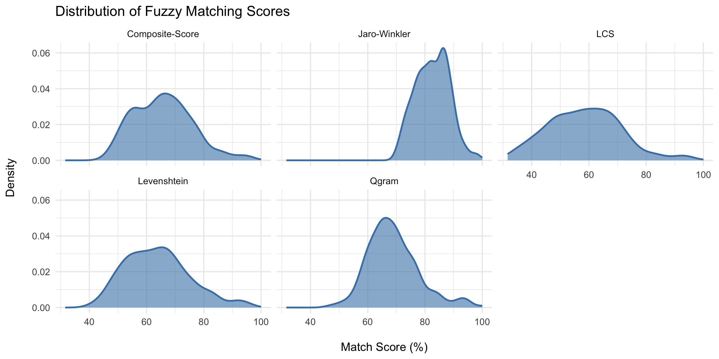
Step 7.1: Visualize score distributions across methods
Before getting into structural evaluations, it’s useful to inspect how the distribution of match scores varies across algorithms. This helps assess whether some methods consistently assign higher scores, and whether their matches tend to cluster tightly or are more dispersed.
This can be particularly important if you intend to apply score thresholds, or want to understand how lenient or strict a method is in assigning high-confidence scores.
Show the code
# plot score dist across methods
all_best |>
  dplyr::filter(method != "Rank-Ensemble") |>
  ggplot2::ggplot(ggplot2::aes(x = score)) +
  ggplot2::geom_density(fill = "steelblue", alpha = 0.6) +

  ggplot2::facet_wrap(~method) +
  ggplot2::geom_density(color = "steelblue", linewidth = 1) +
  ggplot2::labs(
    title = "Distribution of Fuzzy Matching Scores",
    x = "\nMatch Score (%)",
    y = "Density\n"
  ) +
  ggplot2::theme_minimal(base_size = 14)

# save plot
ggplot2::ggsave(
  plot = map_u5mr,
  filename = here::here("03_output/3a_figures/u5mr_sle_adm2.png"),
  width = 12,
  height = 9,
  dpi = 300
)
NoteOutput
To adapt the code:
- Do not modify anything in this section
Looking at the plots, a tight, high peak near 100 means a method produces many strong matches, a broader or flatter distribution may indicate more uncertainty and bimodal patterns may suggest a mix of clearly good and ambiguous matches. These patterns help guide our matching strategy: for our final selection in Step 6, we’ll use an 85% threshold as a starting point and build a fallback system that leans on the most reliable methods first.
Step 7.2: Define match quality diagnostic function
To evaluate the structural quality of a match, we define a simple diagnostic function that compares two names at the token level. It splits each name into individual words (which we will call tokens, since not everything in the name is a word), then does four things:
- checks whether the first words align (prefix match)
- checks whether the last words align (suffix match)
- calculates the difference in word count (token difference)
- calculates the difference in character length (character difference) These simple heuristics can catch mismatches that score high but are structurally off.
assess_match_quality <- function(name1, name2) {
  purrr::map2_dfr(name1, name2, function(a, b) {
    tokens1 <- strsplit(a, "\\s+")[[1]]
    tokens2 <- strsplit(b, "\\s+")[[1]]
    tibble::tibble(
      prefix_match = tolower(tokens1[1]) == tolower(tokens2[1]),
      suffix_match = tolower(tail(tokens1, 1)) == tolower(tail(tokens2, 1)),
      token_diff = abs(length(tokens1) - length(tokens2)),
      char_diff = abs(nchar(a) - nchar(b))
    )
  })
}

assess_match_quality("Makeni Govt Hospital", "Makeni Government Hospital")To adapt the code:
- Do not modify anything in this section
In this example, using our assess_match_quality function, the first and last words match, so both prefix_match and suffix_match are TRUE. There is no difference in the number of tokens (token_diff = 0), but the second name is six characters longer (char_diff = 6) due to “Govt” vs “Government”.
These diagnostics help flag cases where a fuzzy score may be high but important name elements differ, such as CHC vs MCHP, Clinic vs Hospital, or Primary vs Secondary, which can signal a mismatch worth reviewing.
Step 7.3: Evaluate quality of top fuzzy matches
We now run this diagnostic on our best matches. The goal is to highlight cases where, despite high similarity scores, names may differ significantly in format or structure: for example, mismatched prefixes or suffixes. This step supports manual review or adds a layer of filtering to improve final match accuracy.
We also combine the diagnostics into a structure_score (0–100), giving 30% weight to token difference, 20% to character difference, and 25% each to prefix and suffix matches. This provides a quick summary of overall structural alignment.
Show the code
# assess structural match quality
diagnostics_df <- dplyr::bind_cols(
  all_best,
  assess_match_quality(all_best$hf_dhis2, all_best$hf_mfl)
)

# compare method diagnostics
summary_stats <- diagnostics_df |>
  dplyr::group_by(method) |>
  dplyr::summarise(
    score = mean(score),
    avg_token_diff = mean(token_diff) |> round(2),
    avg_char_diff = mean(char_diff) |> round(2),
    pct_prefix_match = (mean(prefix_match) * 100) |> round(2),
    pct_suffix_match = (mean(suffix_match) * 100) |> round(2),
    total = dplyr::n(),
    .groups = "drop"
  )

# create a a final overall score
summary_stats <-  summary_stats |>
  dplyr::mutate(
    # rescale negative of average token difference (smaller is better)
    token_score = scales::rescale(-avg_token_diff, to = c(0, 100)),
    # rescale negative of average character difference (smaller is better)
    char_score = scales::rescale(-avg_char_diff, to = c(0, 100)),
    # rescale prefix match percentage (higher is better)
    prefix_score = scales::rescale(pct_prefix_match, to = c(0, 100)),
    # rescale suffix match percentage (higher is better)
    suffix_score = scales::rescale(pct_suffix_match, to = c(0, 100)),

    # combine all four metrics into a weighted structural quality score
    structure_score = round(
      0.3 * token_score +         # Emphasize fewer token differences
        0.2 * char_score +        # Moderate weight on character similarity
        0.25 * prefix_score +     # Give weight to matching initial words
        0.25 * suffix_score,      # Give equal weight to matching final words
      1
    )
  ) |>
  dplyr::arrange(desc(structure_score)) |>
  # assign rank based on descending structure score
  dplyr::mutate(rank = dplyr::row_number()) |>
  dplyr::select(
    method, avg_token_diff, avg_char_diff,
    pct_prefix_match, pct_suffix_match,
    total, structure_score, rank
  )


# check results
summary_stats |>
  dplyr::select(
    Method = method,
    `Avg. Token Difference` = avg_token_diff,
    `Avg. Character Difference` = avg_char_diff,
    `% Prefix Match` = pct_prefix_match,
    `% Suffix Match` = pct_suffix_match,
    `Structural Score` = structure_score,
      Rank = rank
) |> as.data.frame()To adapt the code: - Lines 32–36: You may adjust the weights used to calculate the structure_score if your matching context values certain components (e.g., prefix matches or token length) more than others
These diagnostics show how well each method preserves the structure of matched names in our example health facility name matching exercise. This helps guide which method to trust most and how to build fallback rules when multiple methods are combined. Your context may result in a different fuzzy matching algorithm being preferred.
Method Performance Summaries
Levenshtein: Lowest token and character differences, with strong prefix and suffix alignment. Highest structural score (84.1, Rank 1) – best overall performer.
Rank-Ensemble: Balanced across metrics, particularly strong on prefix alignment. Score 71.0 (Rank 2) – reliable fallback option.
Composite-Score: Consistent across metrics with solid suffix alignment. Score 68.5 (Rank 3) – flexible, general-purpose option.
Jaro-Winkler: Strongest prefix alignment but weaker on suffixes. Score 67.1 (Rank 4) – useful when beginnings of names align closely.
Qgram: Good at substring similarity, but weaker structurally overall. Score 50.0 (Rank 5) – more suitable for partial overlaps.
LCS Larger token and character gaps despite reasonable suffix matches. Lowest score (43.9, Rank 6) – penalized for structural differences.
Levenshtein was the strongest method, showing low structural differences and good prefix/suffix alignment. Rank-Ensemble and Jaro-Winkler followed as dependable options, with different strengths on prefixes. Composite-Score was steady but slightly weaker. Qgram and LCS were less effective overall, penalized for larger structural gaps despite occasional suffix strengths.
Step 7.4: Weighted thresholding using structural quality and false-positive risk
Now that the structure score is in place, it can be used to calculate additional metrics that strengthen the matching approach. These metrics can feed into a weighted thresholding process, where scores are adjusted by method quality and thresholds are tailored to the false-positive risk of each method. This shifts the threshold setting from a single arbitrary cutoff to an evidence-based process that reflects the strengths and weaknesses of each algorithm, improving precision without sacrificing matching quality.
The outputs from this step serve different purposes depending on your chosen matching strategy in Step 8. If you plan to use a single method or simple composite approach (Options 1-2), you only need the structure score rankings from Step 7.3 to identify the best-performing method. However, if you want to use weighted composite scoring or the fallback loop approach (Options 3-4), you’ll need both the method weights and thresholds calculated in this step.
This step calculates two key metrics for each fuzzy matching method:
1. Method weights: Proportional to structure scores from Step 7.3, rescaled so all weights sum to 1. Methods with better structural quality get higher influence when combining multiple methods in Options 3-4.
2. Method-specific thresholds: Use inverse scaling based on structural quality. A threshold determines the minimum similarity score required for a match (e.g., threshold 85 means only candidates scoring ≥85 are accepted). High-performing methods get lower thresholds (easier matching) because they are reliable, while low-performing methods get higher thresholds (stricter matching) to prevent false positives. For example, Levenshtein might get threshold 75 (trusted method), while LCS gets 95 (requires high confidence).
Note In the code below, the thresholds are created by rescaling each method’s structure_score (0–100) into a new range defined by the 70th and 95th percentiles of all_best$score. The rev() function flips this mapping so that higher scores are pushed toward the lower end of the range and lower scores toward the higher end. This means stronger methods receive stricter thresholds, while weaker methods are assigned looser thresholds.
# calculate method-specific weights and thresholds
method_threshold <- summary_stats |>
  dplyr::mutate(
    score = structure_score / 100,
    weight = score / sum(score),
    threshold = scales::rescale(
      structure_score,
      to = rev(unname(
        stats::quantile(all_best$score, c(0.70, 0.95), na.rm = TRUE)
      ))
    ) |>
      round()
  ) |>
  dplyr::select(method, weight, threshold)

# display results
method_thresholdTo adapt the code:
- Line 1: Keep
summary_statsfrom Step 7.3 with thestructure_scorecolumn - Lines 5–7: Adjust the quantile range (default: 0.70 to 0.95) to control threshold spread
- Line 10: Modify column selection if you need additional metrics in the output
This table shows each method’s relative weight, scaled so all weights sum to one, and its method-specific score threshold derived from observed performance. The relationship between structural quality, weights, and thresholds follows this pattern:
| Method | Weight | Threshold | Interpretation |
|---|---|---|---|
| Levenshtein | 0.219 | 75 | Highest-performing method: gets most influence in composite scoring and lowest threshold for matching |
| Composite-Score | 0.185 | 80 | Strong performer: high influence and low threshold |
| Rank-Ensemble | 0.178 | 81 | Good performer: moderate-high influence and low-medium threshold |
| Jaro-Winkler | 0.174 | 82 | Balanced method: moderate influence and medium threshold |
| Qgram | 0.130 | 88 | Lower performer: reduced influence and higher threshold to prevent false positives |
| LCS | 0.114 | 92 | Lowest performer: minimal influence and strictest threshold required |
Key insight: Methods with better structural alignment get rewarded with higher weights (more influence) and lower thresholds (easier matching), while unreliable methods are constrained with lower weights and stricter thresholds.
Step 8: Finalize Fuzzy Match Selection
This step assigns a final match to each DHIS2 facility by choosing the most appropriate candidate from the fuzzy matching results. At this stage, every unmatched facility from earlier steps should have a set of one or more candidate matches with similarity scores and any supporting diagnostics (e.g., prefix/suffix matches, token differences). The goal is to select one match per facility in a way that balances accuracy, efficiency, and coverage.
The choice of final selection strategy depends on:
- Confidence in your matching methods: If your algorithms and thresholds are already well-tuned to the data, you can use a simpler approach.
- Tolerance for false positives: In some contexts, a slightly lower match rate is acceptable if it reduces the risk of incorrect matches.
- Analytical and operational priorities: For example, whether you need a quick, explainable method for an urgent report, or a more comprehensive, iterative process for a master dataset update.
We offer four structured options, each with its own strengths, weaknesses, and level of complexity. In practice, you may start with a simpler option and progress to more advanced approaches if too many facilities remain unmatched or if match quality is inconsistent. These options are also compatible with an SNT team review step, allowing human validation before matches are finalized in the dataset.
Summary of Match Selection Options
| Option | Description | Use Case | Code Complexity |
|---|---|---|---|
| Option 1: Single Method | Use one preferred method (e.g., Levenshtein) with a threshold | When confident in a single algorithm | Low |
| Option 2: Composite/Rank | Use composite score or rank average to select best match | When using blended match signals | Moderate |
| Option 3: Weighted Composite Score | Use performance-weighted composite score that accounts for method reliability and false-positive rates | When using blended match signals with known method performance differences | Moderate |
| Option 4: Fallback Loop | Stepwise fallback through all methods based on structural quality scores | When coverage is most important | High |
Step 8.1: Match selection options
Option 1: Single Preferred Method
This approach uses one similarity algorithm, such as Levenshtein or Jaro-Winkler, to select the highest-scoring match for each facility. The analyst applies a fixed threshold so that scores above the cut-off are accepted as matches, while the system flags lower scores for review. It is fast, easy to explain, and works well when the chosen method aligns with the types of name differences in your data.
Show the code
# apply single-method threshold and flag matches
best_lv_final <- best_lv |>
  dplyr::mutate(
    match_flag = dplyr::if_else(score >= 85, "match", "review"),
    final_method = "Levenshtein"
  ) |>
  dplyr::left_join(
    dplyr::select(master_hf_df, hf_mfl, hf_mfl_raw),
    by = "hf_mfl"
  ) |>
  dplyr::select(hf_dhis2, hf_mfl, hf_mfl_raw, score, final_method, match_flag)

# show top 5 and bottom 5 matches by score
top_5 <- best_lv_final |>
  dplyr::arrange(dplyr::desc(score)) |>
  dplyr::slice_head(n = 5)

bottom_5 <- best_lv_final |>
  dplyr::arrange(score) |>
  dplyr::slice_head(n = 5)

# combine into a single table
top_bottom <- dplyr::bind_rows(top_5, bottom_5)

cli::cli_h3("Top 5 and Bottom 5 Matches by Levenshtein Score")

# preview results
top_bottomTo adapt the code:
- Line 2: Replace
best_lvwith another object from Step 4.5 (e.g.,best_jw,best_qg) depending on your preferred method - Line 4: Adjust the score threshold (default = 85) to define what is considered a
match - Line 6: Keep column names
hf_dhis2andhf_mfl, or replace them with your own
In our example dataset, the Levenshtein method with an 85% threshold achieved the match rate shown in the output above. This conservative approach prioritizes precision over recall, making it suitable when false positives are costly and manual review resources are available.
Option 2: Composite or Rank-Based Match
This approach selects the best match using a combined measure from multiple algorithms, such as a composite score or average rank. It avoids relying on a single method while keeping the process simpler than a full fallback loop. This works well when different algorithms capture different types of variation, and a single combined score can be used with a threshold to separate confident matches from those needing review.
Show the code
# select best match using rank average
composite_final <- ranked_grid |>
  dplyr::group_by(hf_dhis2) |>
  dplyr::arrange(rank_avg) |>
  dplyr::slice_head(n = 1) |>
  dplyr::ungroup() |>
  dplyr::mutate(
    match_flag = dplyr::if_else(composite_score >= 85, "match", "review")
  ) |>
  dplyr::select(
    adm1,
    adm2,
    hf_dhis2,
    hf_mfl,
    composite_score,
    rank_avg,
    match_flag
  )

# show top 5 and bottom 5 matches by composite score
top_5 <- composite_final |>
  dplyr::arrange(dplyr::desc(score)) |>
  dplyr::slice_head(n = 5)

bottom_5 <- composite_final |>
  dplyr::arrange(score) |>
  dplyr::slice_head(n = 5)

# combine into a single table
top_bottom <- dplyr::bind_rows(top_5, bottom_5)

cli::cli_h3("Top 5 and Bottom 5 Matches by Composite Score")

# preview results
top_bottomTo adapt the code:
- Line 2: Keep
ranked_gridfrom Step 6.4, or replace with your combined results dataframe - Line 7: Adjust the composite score threshold (default = 85) to define what is considered a
match - Lines 9–14: Keep score columns (
composite_score,rank_avg) or replace with your scoring metrics
The composite score approach results in the match rate shown in the output above. This reflects the averaging effect where strong matches in one method may be diluted by weaker scores in others. Best suited for datasets with consistent naming patterns across methods.
Option 3: Weighted Composite Score
This approach selects the best match using a performance-weighted composite score that accounts for method reliability and false-positive rates. Instead of treating all methods equally, it uses the weights calculated in Step 7.4 to emphasize methods that demonstrated better structural alignment. This provides a more sophisticated alternative to simple averaging while being less complex than a full fallback system.
The weighted composite score uses a weighted average that maintains the 0-100 scale: Methods with higher structural quality scores get more weight in the final composite. For example, if Levenshtein has weight 0.4 and Qgram has weight 0.1, the Levenshtein score contributes 4x more to the final weighted score.
Show the code
# define score columns and extract weights
score_cols <- c("score_jw", "score_lv", "score_qg", "score_lcs")

weights <- method_threshold |>
  dplyr::filter(
    method %in% c("Jaro-Winkler", "Levenshtein", "Qgram", "LCS")
  ) |>
  dplyr::pull(weight)

# calculate weighted composite score for each facility-match pair
weighted_final <- ranked_grid |>
  dplyr::rowwise() |>
  dplyr::mutate(
    # weighted average maintains 0-100 scale
    weighted_composite_score = stats::weighted.mean(
      c(score_jw, score_lv, score_qg, score_lcs),
      weights,
      na.rm = TRUE
    )
  ) |>
  dplyr::ungroup() |>
  dplyr::group_by(hf_dhis2) |>
  dplyr::arrange(dplyr::desc(weighted_composite_score)) |>
  dplyr::slice_head(n = 1) |>
  dplyr::ungroup() |>
  dplyr::mutate(
    match_flag = dplyr::if_else(
      weighted_composite_score >= 85,
      "match",
      "review"
    ),
    score = weighted_composite_score, # standardize column name for Step 7
    final_method = "Weighted-Composite"
  ) |>
  dplyr::left_join(
    dplyr::select(master_hf_df, hf_mfl, hf_mfl_raw),
    by = "hf_mfl"
  ) |>
  dplyr::select(
    hf_dhis2,
    hf_mfl,
    hf_mfl_raw,
    score,
    final_method,
    match_flag
  )

# show top 5 and bottom 5 matches by weighted composite score
top_5 <- weighted_final |>
  dplyr::arrange(dplyr::desc(score)) |>
  dplyr::slice_head(n = 5)

bottom_5 <- weighted_final |>
  dplyr::arrange(score) |>
  dplyr::slice_head(n = 5)

cli::cli_h3("Top 5 and Bottom 5 Matches by Weighted Composite Score")

# preview results
bottom_5To adapt the code:
- Line 2: Adjust
score_colsif you have different similarity score columns in your dataset - Lines 4–8: Ensure
method_thresholdfrom Step 7.4 contains weights for the methods you’re using - Lines 15–18: The
weighted.mean()function calculates a weighted average that maintains the 0-100 scale - Lines 24–27: Adjust the weighted composite score threshold (default = 85) to define what is considered a
match - Lines 36–41: Select columns to include in the final output
The weighted composite approach achieved the improved match rate shown in the output above. This improvement over the simple composite demonstrates the value of emphasizing high-quality methods. The weighting balances the strengths of multiple models while prioritizing the most reliable algorithms.
Option 4: Fallback Loop Across Methods (Recommended for Coverage)
This approach maximizes match coverage through a sophisticated tiered fallback system that dynamically uses the method ordering and thresholds calculated in Steps 7.3 and 7.4. Methods are applied in descending order of their structure scores, ensuring high-precision algorithms get the first chance to match.
A key strength is the use of method-specific thresholds from Step 7.4. Each method uses its own calculated threshold based on its structural quality and false-positive risk profile. This evidence-based approach is more reliable than arbitrary cutoffs.
The method order and thresholds are dynamically determined from the structural quality analysis in Steps 7.3-7.4. Methods with higher structure scores are prioritized, and each uses its calculated threshold based on false-positive risk:
- High-quality methods (e.g., Levenshtein): Lower thresholds due to reliable matching
- Medium-quality methods (e.g., Jaro-Winkler): Moderate thresholds for balanced precision
- Lower-quality methods (e.g., Qgram, LCS): Higher thresholds to prevent false positives
The fallback process works as follows:
- Method ordering: Methods are ordered by their structure scores from Step 7.3 (highest to lowest)
- Tie-breaking: Within each method, candidates are pre-sorted by:
- Similarity score (descending) - highest scores first
- Average rank from ensemble methods (ascending) - best ranks as secondary criterion This ensures that when multiple candidates exceed the threshold, the best match is selected
- Progressive matching: Each method attempts to match remaining facilities using its calculated threshold from Step 7.4
- Threshold relaxation: If facilities remain unmatched after a full pass, thresholds are reduced by 1 point and the cycle repeats
- Quality floor: Process stops when all facilities are matched or thresholds drop below 50
This dynamic approach with robust tie-breaking ensures the best possible match for each facility while maintaining quality standards based on empirical performance metrics.
Show the code
# extract method order and thresholds from step 7.4 results
# order methods by structure score (highest to lowest)
method_stats <- summary_stats |>
  dplyr::arrange(dplyr::desc(structure_score)) |>
  dplyr::filter(method != "Rank-Ensemble") # exclude rank-based method

method_order <- method_stats$method

# use thresholds calculated in step 7.4
method_thresholds_df <- method_threshold |>
  dplyr::filter(method != "Rank-Ensemble")

# convert to named vector for easy lookup
method_thresholds <- setNames(
  method_thresholds_df$threshold,
  method_thresholds_df$method
)

# build combined table of top matches from real methods only
all_best_nonrank <- dplyr::bind_rows(
  best_lv,
  best_jw,
  best_qg,
  best_lcs,
  best_comp
) |>
  # normalize method labels
  dplyr::mutate(method = trimws(method))

# add rank once
rank_key <- ranked_grid |>
  dplyr::select(hf_dhis2, hf_mfl, rank_avg)

all_best_ranked <- all_best_nonrank |>
  dplyr::left_join(rank_key, by = c("hf_dhis2", "hf_mfl")) |>
  dplyr::mutate(
    # worst for missing ranks
    rank_avg = dplyr::if_else(is.na(rank_avg), Inf, rank_avg)
  )

# split by method and pre-arrange for stable tiebreak
by_method <- split(all_best_ranked, all_best_ranked$method) |>
  purrr::map(\(x) {
    x |>
      dplyr::arrange(dplyr::desc(score), rank_avg)
  })

# keep copy for pass-rate check
initial_thr <- method_thresholds

# init
fallback_chunks <- list()
unmatched <- unique(all_best_ranked$hf_dhis2)

# fast fallback loop (no joins, no grouping inside)
repeat {
  for (m in method_order) {
    if (!m %in% names(by_method)) {
      next
    }

    # current threshold from step 7.4
    thr <- method_thresholds[[m]]
    if (is.null(thr)) {
      thr <- 85 # fallback if method not found
    }

    # filter by score and still-unmatched
    cand <- by_method[[m]] |>
      dplyr::filter(score >= thr, hf_dhis2 %in% unmatched)

    if (nrow(cand) > 0) {
      # pick first row per hf_dhis2 (pre-arranged by score desc, rank asc)
      best_per_hf <- cand |>
        dplyr::distinct(hf_dhis2, .keep_all = TRUE) |>
        dplyr::mutate(
          final_method = glue::glue("Fuzzy-matched using: {m}")
        )

      # store and update unmatched
      fallback_chunks[[length(fallback_chunks) + 1L]] <- best_per_hf
      unmatched <- setdiff(unmatched, best_per_hf$hf_dhis2)
    }

    if (length(unmatched) == 0) break
  }

  if (length(unmatched) == 0) {
    break
  }

  # relax thresholds gradually
  method_thresholds <- method_thresholds - 1
  if (any(method_thresholds <= 50)) break # stop if too low
}

# bind once
fallback_matched <- dplyr::bind_rows(fallback_chunks)

# build a 1:1 map from standardized DHIS2 name to admin + raw +
# hf_uid_new
hf_uid_new_map_by_stand <- dhis2_hf_unmatched |>
  dplyr::arrange(adm0, adm1, adm2, adm3, hf_dhis2_raw) |>
  dplyr::group_by(hf_dhis2) |>
  dplyr::summarise(
    adm0 = dplyr::first(adm0),
    adm1 = dplyr::first(adm1),
    adm2 = dplyr::first(adm2),
    adm3 = dplyr::first(adm3),
    hf_dhis2_raw = dplyr::first(hf_dhis2_raw),
    hf_uid_new = dplyr::first(hf_uid_new),
    .groups = "drop"
  )

# final flags and attach admin + ids
fallback_final <- fallback_matched |>
  dplyr::mutate(
    match_flag = dplyr::if_else(score >= 85, "match", "review")
  ) |>
  dplyr::left_join(
    dplyr::select(master_hf_df, hf_mfl, hf_mfl_raw),
    by = "hf_mfl"
  ) |>
  dplyr::left_join(hf_uid_new_map_by_stand, by = "hf_dhis2") |>
  dplyr::select(
    adm0, adm1, adm2, adm3,
    hf_uid_new,
    hf_dhis2_raw,
    hf_dhis2,
    hf_mfl_raw,
    hf_mfl,
    score,
    final_method,
    match_flag
  )

top_5 <- fallback_final |>
  dplyr::arrange(dplyr::desc(score)) |>
  dplyr::slice_head(n = 5)

bottom_5 <- fallback_final |>
  dplyr::arrange(score) |>
  dplyr::slice_head(n = 5)

cli::cli_h3("Top 5 and Bottom 5 Matches by Fallback")

bottom_5 <- dplyr::bind_rows(top_5, bottom_5)

# preview results
bottom_5To adapt the code:
- Lines 2–8: The method order is automatically determined from
summary_statsstructure scores - Lines 9–16: Thresholds are extracted from Step 7.4’s
method_thresholddataframe - Line 65: The fallback threshold (default = 85) is used only if a method lacks a calculated threshold
- Line 94: The minimum threshold (default = 50) prevents accepting very low-quality matches
- Lines 33, 36, throughout: Replace
hf_dhis2andhf_mflwith your dataset’s column names if they differ
The fallback loop achieved the highest match rate as shown in the output above. This substantial improvement over other methods demonstrates the effectiveness of method-specific thresholds and progressive fallback. The approach maximizes coverage while maintaining quality through data-driven thresholds and intelligent tie-breaking.
This is the approach that we will use going forward, as it offers the best balance between coverage and match quality, reduces the manual review workload, and adapts thresholds dynamically to the strengths and weaknesses of each method.
Step 8.2: Select fuzzy matching approach
After reviewing the different fuzzy matching options from Step 8.1, select which approach to use in your final workflow. This step creates the fuzzy_matches dataset that will be combined with other matching methods in Step 9.
NoteChoosing Your Approach
Select one approach based on your evaluation in Step 8.1: - Use single algorithm (Levenshtein, Jaro-Winkler, or Q-gram) for simplicity and interpretability - Use composite scores when you want to balance multiple algorithms - Use weighted approach when domain expertise suggests certain algorithms are more reliable for your data - Use fallback approach for the most comprehensive matching with hierarchical scoring
Show the code
# create fuzzy_matches from step 8 results (use whichever option was
# chosen)
# step 8 produces different result datasets depending on which option
# was
# chosen:
# - option 1: best_lv_final, best_jw_final, etc.
# - option 2: composite_final
# - option 3: weighted_final
# - option 4: fallback_final

fuzzy_matches <- if (exists("fallback_final")) {
  dplyr::filter(fallback_final, match_flag == "match")
} else if (exists("composite_final")) {
  dplyr::filter(composite_final, match_flag == "match")
} else if (exists("weighted_final")) {
  dplyr::filter(weighted_final, match_flag == "match")
} else if (exists("best_lv_final")) {
  dplyr::filter(best_lv_final, match_flag == "match")
} else if (exists("best_jw_final")) {
  dplyr::filter(best_jw_final, match_flag == "match")
} else if (exists("best_qg_final")) {
  dplyr::filter(best_qg_final, match_flag == "match")
} else {
  # empty dataframe with expected structure if no step 8 results exist
  data.frame(
    hf_dhis2_raw = character(0),
    hf_dhis2 = character(0),
    hf_mfl_raw = character(0),
    hf_mfl = character(0),
    score = numeric(0),
    final_method = character(0),
    stringsAsFactors = FALSE
  )
} |>
# remove any internal duplicates (keep highest scoring match per
# facility)
dplyr::group_by(hf_dhis2_raw) |>
dplyr::slice_max(score, n = 1, with_ties = FALSE) |>
dplyr::ungroup() |>
# attach admin + hf_uid_new from unmatched (collapse to 1:1 per
# hf_dhis2_raw)
{
  hf_uid_new_map_unmatched <- dhis2_hf_unmatched |>
    dplyr::arrange(adm0, adm1, adm2, adm3, hf_dhis2_raw) |>
    dplyr::group_by(hf_dhis2_raw) |>
    dplyr::summarise(
      adm0 = dplyr::first(adm0),
      adm1 = dplyr::first(adm1),
      adm2 = dplyr::first(adm2),
      adm3 = dplyr::first(adm3),
      hf_uid_new = dplyr::first(hf_uid_new),
      .groups = "drop"
    )
  dplyr::left_join(., hf_uid_new_map_unmatched, by = "hf_dhis2_raw")
}

# display summary of selected approach
cli::cli_h2("Selected Fuzzy Matching Results")
cli::cli_alert_success("Fuzzy matches found: {nrow(fuzzy_matches)}")

if (nrow(fuzzy_matches) > 0) {
  score_summary <- fuzzy_matches |>
    dplyr::summarise(
      avg_score = mean(score, na.rm = TRUE),
      min_score = min(score, na.rm = TRUE),
      max_score = max(score, na.rm = TRUE),
      .groups = "drop"
    )

  cli::cli_alert_info("Score range: {round(score_summary$min_score, 1)} - {round(score_summary$max_score, 1)}")
  cli::cli_alert_info("Average score: {round(score_summary$avg_score, 1)}")
}To adapt the code:
- Lines 6-20: The conditional logic checks for different Step 8 result datasets in priority order. Modify the order if you prefer a different approach to take precedence
- Lines 21-29: Create empty dataframe structure if no Step 8 results exist. Ensure column names match your expected structure
- Lines 31-34: Deduplication logic removes internal duplicates within the selected approach, keeping the highest scoring match per DHIS2 facility. Modify if you need different deduplication rules
- Alternative approach: Instead of conditional logic, you can directly assign your chosen dataset: ````
Step 8.3: Manual review of flagged matches
Before finalizing matches and joining back to your main datasets, all records flagged as review must be manually validated or rejected by the SNT team or designated reviewers. This step ensures data quality and prevents false positives from entering the analysis.
ImportantConsult with SNT team
Manual review is required for all review matches before proceeding to Step 9. The SNT team should confirm or reject uncertain matches and document patterns in false positives or missed matches to refine future matching workflows.
Preparing Data for Manual Review
Below, we export review matches to a structured file for systematic checking:
Show the code
# prepare review dataset (using fallback results as example)
review_matches <- fallback_final |>
  dplyr::filter(match_flag == "review") |>
  dplyr::arrange(dplyr::desc(score)) |>
  dplyr::mutate(
    reviewer_decision = NA_character_, # accept/reject/uncertain
    reviewer_notes = NA_character_,
    review_date = NA_character_,
    reviewer_name = NA_character_
  ) |>
  dplyr::select(
    adm0, adm1, adm2, adm3, hf_uid_new,
    hf_dhis2_raw,
    hf_dhis2,
    hf_mfl_raw,
    hf_mfl,
    score,
    final_method,
    reviewer_decision,
    reviewer_notes,
    review_date,
    reviewer_name
  )

# export for review
readr::write_csv(
  review_matches,
  here::here("03_outputs", "tables", "facility_matches_for_review.csv")
)

# show summary
cli::cli_h2("Manual Review Required")
cli::cli_alert_info(
  "Exported {nrow(review_matches)} matches flagged for review"
)
cli::cli_alert_info(
  "File location: outputs/facility_matches_for_review.csv"
)To adapt the code:
- Lines 6–12: Add additional columns for your review process (e.g., facility_type, district)
- Line 15: Adjust the output file path and name as needed
Review Process Guidelines
The manual review step is more than a simple yes/no decision. It is an opportunity to strengthen the matching workflow by confirming accurate links, rejecting false positives, and documenting recurring data quality issues. Reviewers play a key role in ensuring the integrity of the final dataset and in improving the process for future runs.
For Reviewers:
- Accept – Confirm that both names refer to the same facility. Look for strong evidence of equivalence, such as:
- Minor spelling variations:
"Makeni Gov Hospital"↔︎"Makeni Government Hospital" - Common or consistent abbreviations:
Bo CHC↔︎Bo Community Health Center - Small formatting differences that do not alter meaning
- Minor spelling variations:
- Reject – Flag cases where facilities differ or where the match is too uncertain. Common examples include:
- Different facility types in the same area:
"Makeni Hospital"↔︎"Makeni Clinic" - Generic names without geographic qualifiers:
Community Health Postwithout a location - Multiple possible matches in the same vicinity without clear identifiers
- Different facility types in the same area:
- Document patterns – Use the review to capture recurring issues. These insights help refine thresholds, weights, and matching rules. Examples:
- Frequent abbreviation mismatches (e.g.,
CHCvsCH Centre) - Regional or language-specific naming conventions
- Missing or inconsistent administrative unit data in source systems
- Frequent abbreviation mismatches (e.g.,
A systematic approach to review ensures that accepted matches are trustworthy, rejected matches are well-justified, and lessons learned feed directly into improving the next matching cycle.
Simulated Review Decisions
For demonstration purposes, we simulate reviewer decisions on the flagged matches. In practice, this would be done by domain experts reviewing the exported CSV file.
After manual review is complete, we import the data that has all the decisions.
Show the code
# simulate reviewer decisions (replace with actual reviewed data)
# read back reviewed matches
reviewed_matches <- readr::read_csv(
  here::here("03_outputs", "tables", "facility_matches_reviewed.csv"),
  col_types = readr::cols(
    reviewer_decision = readr::col_character(),
    reviewer_notes = readr::col_character(),
    review_date = readr::col_character(),
    reviewer_name = readr::col_character()
  )
)
To adapt the code:
- Line 3: Update the file path to your project’s output directory
- Lines 4–8: Add additional column types if your review file includes extra fields
Incorporating Review Results
Now we integrate the reviewer decisions back into your matching workflow:
Show the code
final_incorp <- reviewed_matches |>
  dplyr::mutate(
    final_match_flag = dplyr::case_when(
      reviewer_decision == "accept" ~ "match",
      reviewer_decision == "reject" ~ "no_match",
      is.na(reviewer_decision) ~ "pending_review",
      TRUE ~ "no_match"
    )
  )

# get the final matched ones
final_matches <- final_incorp |>
  dplyr::filter(final_match_flag == "match") |>
  dplyr::select(-reviewer_decision)

# summary of all results (including rejected/pending)
all_results_summary <- final_incorp |>
  dplyr::count(final_match_flag, name = "n") |>
  dplyr::mutate(percentage = round(100 * n / sum(n), 1))

# summary of final accepted matches only
final_summary <- final_matches |>
  dplyr::count(final_match_flag, name = "n")

cli::cli_h2("Final Matching Results After Manual Review")
cli::cli_alert_success(
  "Accepted matches: {format(sum(final_summary$n), big.mark = ',')}"
)

# breakdown by decision type
rejected_count <- all_results_summary |>
  dplyr::filter(final_match_flag == "no_match") |>
  dplyr::pull(n)
if (length(rejected_count) == 0) {
  rejected_count <- 0
}

pending_count <- all_results_summary |>
  dplyr::filter(final_match_flag == "pending_review") |>
  dplyr::pull(n)
if (length(pending_count) == 0) {
  pending_count <- 0
}

if (rejected_count > 0) {
  cli::cli_alert_danger(
    "Rejected matches: {format(rejected_count, big.mark = ',')} (will have NA MFL values in final dataset)"
  )
}

if (pending_count > 0) {
  cli::cli_alert_warning(
    "Pending review: {format(pending_count, big.mark = ',')} (require additional review)"
  )
}

# show breakdown table
all_results_summaryTo adapt the code:
- Line 3: Update the file path from
"03_outputs"to your project’s output directory - Lines 4–8: Add additional column types if your review file includes extra fields
- Lines 12–18: Adjust logic for handling different reviewer decision categories based on your workflow
Out of the 159 proposed matches, none were accepted, as all appeared to be different. This may suggest underlying data quality issues or the presence of new health facility names.
DHIS2 facilities with rejected matches will appear in the final dataset (Step 9) with NA values for MFL columns, preserving the facility record while clearly indicating no reliable match was found. Facilities with pending review should be resolved before proceeding to production use.
Step 9: Combine All Matched Results
In this step, we combine results from all matching approaches and finalize the dataset by joining back to the original DHIS2 health facility list. This creates a comprehensive dataset that includes:
- High-confidence matches from Step 4 (Interactive Stratified Geographic Matching)
- Fuzzy matches from Step 6-8 (Various fuzzy matching strategies on remaining unmatched)
- Unmatched facilities (Preserved with NA values for MFL columns)
Step 9.1: Combine results from all matching approaches
When using the enhanced workflow with stratified matching, combine results from all stages:
Show the code
# create manual_matches from manual review results (both matched and
# unmatched)
manual_matches <- final_incorp |>
  dplyr::mutate(
    # for unmatched, set appropriate values
    hf_mfl = dplyr::if_else(
      reviewer_decision == "accept",
      hf_mfl,
      NA_character_
    ),
    hf_mfl_raw = dplyr::if_else(
      reviewer_decision == "accept",
      hf_mfl_raw,
      NA_character_
    ),
    final_method = dplyr::if_else(
      reviewer_decision == "accept",
      "Manual Review - Accepted",
      "Manual Review - Rejected"
    ),
    score = dplyr::if_else(
      reviewer_decision == "accept",
      100,
      0
    )
  ) |>
  # manual reviewed results already carry adm0-3 + hf_uid_new from
  # fallback_final → review export → reimport
  dplyr::select(
    adm0,
    adm1,
    adm2,
    adm3,
    hf_uid_new,
    hf_dhis2_raw,
    hf_dhis2,
    hf_mfl_raw,
    hf_mfl,
    score,
    final_method
  )

# combine results from all matching approaches
# this dataset contains ALL facilities: matched, unmatched, and
# rejected
final_facilities_all <- dplyr::bind_rows(
  matched_dhis2_prepgeoname, # Step 4: Stratified geographic matches (if performed)
  matched_dhis2, # Step 5: Exact matches after standardization
  fuzzy_matches, # Step 6-8: Complete matches from fuzzy matching
  manual_matches # Manual matching (if performed)
)

# collapse to one record per DHIS2 facility for downstream integration
final_facilities_one_per_hf <- final_facilities_all |>
  dplyr::select(-match_flag, -hf)

cli::cli_alert_info(
  "All facilities processed (rows): {nrow(final_facilities_all)}"
)
cli::cli_alert_success(
  "All facilities processed (distinct DHIS2 by adm0/1/2/3+hf): {dplyr::n_distinct(final_facilities_all$hf_uid_new)}"
)

# generate summary by matching method
matching_summary <- final_facilities_one_per_hf |>
  dplyr::group_by(final_method) |>
  dplyr::summarise(
    n_matched = n(),
    avg_score = mean(score, na.rm = TRUE),
    min_score = min(score, na.rm = TRUE),
    max_score = max(score, na.rm = TRUE),
    .groups = "drop"
  )

# display summary
cli::cli_h2("Matching Results by Method")
matching_summaryTo adapt the code:
- Lines 6-13: The
fuzzy_matcheslogic automatically detects which Step 8 approach was used. Modify the order or add additional Step 8 result variables if needed - Lines 15-25: The
manual_matcheslogic processes both matched and rejected facilities fromfinal_incorp. Replacefinal_incorpwith your manual review results dataset name - Lines 19-26: Facilities that were rejected in manual review get
final_method = "Manual Review - Rejected"andscore = 0. Adjust these labels if needed - Lines 28-32: The
bind_rowscombines all matching approaches. Add or remove rows based on which steps you used in your workflow - Lines 33-36: Deduplication logic removes duplicates by keeping the highest scoring match for each DHIS2 facility (grouped by
hf_dhis2_rawonly). Modify if you need different deduplication rules - Lines 38-55: Validation checks detect internal duplicates within each dataset and verify the final combined dataset has no duplicates. Remove or modify these checks if not needed
Step 9.2: Create final integrated DHIS2-MFL dataset
Create the final analytical dataset by starting with DHIS2 as the base and enriching it with MFL data where matches exist. This ensures no DHIS2 facilities are lost while adding valuable MFL attributes.
Show the code
# start with DHIS2 as base to preserve all rows; attach hf_uid_new
dhis2_df_final <- dhis2_df |>
  dplyr::left_join(
    dhis2_map,
    by = c("adm0", "adm1", "adm2", "adm3", "hf")
  )

# one-per-facility matching results: use hf_uid_new as the join key
final_match_per_hf <- final_facilities_one_per_hf |>
  dplyr::select(hf_uid_new, hf_mfl_raw)

# create the integrated dataset
final_dhis2_mfl_df <- dhis2_df_final |>
  dplyr::left_join(final_match_per_hf, by = "hf_uid_new") |>
  # join MFL attributes for matched facilities
  dplyr::left_join(
    dplyr::select(master_hf_df, -hf_mfl, -hf, -adm0, -adm1, -adm2, -adm3),
    by = "hf_mfl_raw"
  )

# counts on distinct facilities via hf_uid_new (robust to row-level
# duplication)
total <- dhis2_df_final |> dplyr::distinct(hf_uid_new) |> nrow()
with_mfl <- final_match_per_hf |>
  dplyr::filter(!is.na(hf_mfl_raw)) |>
  nrow()
without_mfl <- total - with_mfl

# validation summary
cli::cli_h2("DHIS2-MFL Integration Complete")
cli::cli_alert_success(
  "Total DHIS2 facilities preserved: {total}"
)
cli::cli_alert_info(
  "Facilities with MFL data: {with_mfl}"
)
cli::cli_alert_warning(
  "Facilities without MFL match: {without_mfl}"
)
cli::cli_alert_info("Total rows (facility-months): {nrow(final_dhis2_mfl_df)}")To adapt the code:
- Line 7: Change
hfto match your DHIS2 facility name column - Lines 11-12: Adjust which MFL columns to exclude (we remove geographic columns to avoid conflicts with DHIS2’s geography)
- Line 13: Ensure
hf_mfl_rawmatches the MFL facility name column from your matching results
Step 10: Final Checks
Perform critical quality checks before finalizing the matching workflow. This step identifies potential data quality issues that require SNT team review: one-to-many matches (which may indicate duplicate facilities or generic names) and unmatched facilities (which could represent new facilities, closed facilities, or data quality issues). These checks ensure match quality and create actionable review lists for the SNT team.
Step 10.1: Detecting one-to-many matches for review
After finalization, check for MFL facilities matched to multiple DHIS2 facilities, which may indicate data quality issues requiring review:
Show the code
# detect MFL facilities matched to multiple DHIS2 facilities
one_to_many <- final_facilities_all |>
  dplyr::filter(!is.na(hf_mfl_raw)) |> # only matched facilities
  dplyr::group_by(hf_mfl_raw) |>
  dplyr::filter(dplyr::n() > 1) |> # MFL matched to >1 DHIS2
  dplyr::ungroup() |>
  dplyr::arrange(hf_mfl_raw, hf_dhis2_raw)

if (nrow(one_to_many) > 0) {
  cli::cli_alert_warning(
    paste0(
      "One-to-many matches detected: {nrow(one_to_many)} DHIS2 facilities ",
      "share {dplyr::n_distinct(one_to_many$hf_mfl_raw)} MFL facilities"
    )
  )

  # show sample
  knitr::kable(
    one_to_many |>
      dplyr::select(hf_dhis2_raw, hf_mfl_raw, score, final_method) |>
      dplyr::slice_head(n = 6),
    caption = "Sample one-to-many matches requiring review"
  )
} else {
  cli::cli_alert_success("No one-to-many matches detected")
}To adapt the code:
- Line 4: Modify output path for the review file as needed
- Lines 19-23: Adjust which columns to include in the review file
One-to-many matches often signal underlying issues in the data. They may arise from duplicate or near-duplicate facility records in DHIS2, or from generic names in the MFL that align with multiple, more specific DHIS2 entries. In other cases, they reflect inconsistent naming conventions that need further standardization before integration.
Step 10.2: Unmatched facilities analysis
Analyze facilities that remain unmatched to identify potential reasons and create actionable review lists for the SNT team. Unmatched facilities could represent new facilities, closed facilities, or facilities with significant data quality issues.
Show the code
# analyze unmatched facilities by reason
unmatched_analysis <- final_facilities_all |>
  dplyr::filter(is.na(hf_mfl_raw)) |>
  dplyr::group_by(final_method) |>
  dplyr::summarise(
    count = n(),
    .groups = "drop"
  ) |>
  dplyr::arrange(desc(count))

# display unmatched analysis
cli::cli_h2("Unmatched Facilities Analysis")
cli::cli_alert_info(
  "Total unmatched facilities: {sum(unmatched_analysis$count)}"
)

# show breakdown by reason
purrr::pwalk(
  unmatched_analysis,
  ~ cli::cli_alert_warning("{.x}: {.y} facilities")
)

# create detailed unmatched facilities export
unmatched_detailed <- final_facilities_one_per_hf |>
  # unmatched are those without an MFL linkage
  dplyr::filter(is.na(hf_mfl_raw)) |>
  # select required context and scoring/method fields
  dplyr::select(
    hf_dhis2_raw,
    adm1,
    adm2,
    adm3,
    final_method,
    score
  ) |>
  # derive a clear potential reason for review
  dplyr::mutate(
    potential_reason = dplyr::case_when(
      is.na(final_method) ~ "Never matched - possible new facility",
      final_method == "Manual Review - Rejected" ~
        "Rejected in review - possible different facility",
      score > 0 & score < 50 ~ "Low similarity - possible data quality issue",
      TRUE ~ "Unmatched - needs investigation"
    )
  ) |>
  dplyr::arrange(adm1, adm2, adm3, hf_dhis2_raw)

# export for SNT team review
readr::write_csv(
  unmatched_detailed,
  here::here("03_outputs", "unmatched_facilities_for_snt_review.csv")
)

cli::cli_alert_success(
  "Exported {nrow(unmatched_detailed)} unmatched facilities for SNT team review"
)
cli::cli_text("File: outputs/unmatched_facilities_for_snt_review.csv")To adapt the code:
- Lines 3-9: Analysis groups unmatched facilities by reason (final_method). Customize grouping as needed
- Lines 17-32: Detailed export includes geographic context and potential reasons. Modify columns based on your needs
- Lines 34-39: Export path for SNT team review can be customized
- Lines 41-44: The potential reasons logic can be adjusted based on your specific workflow patterns
This check helps the SNT team focus their review on the most important cases. Some unmatched facilities may represent new sites that should be added to the MFL, while others point to data quality issues where name variations need correction. A portion may be closed facilities that need to be marked inactive. The results can also highlight geographic patterns, showing areas where unmatched facilities are more common and may require targeted review.
Step 11: Save Final Datasets
Save all final datasets for analysis, reporting, and SNT team review. This step consolidates all export operations and creates the outputs needed for downstream use.
Show the code
# save main integrated DHIS2-MFL dataset
rio::export(
  final_dhis2_mfl_df,
  here::here("03_outputs", "final_dhis2_mfl_integrated.xlsx")
)

# save matching results summary
rio::export(
  final_facilities_all,
  here::here("03_outputs", "facility_matching_results.xlsx")
)

if (nrow(unmatched_facilities) > 0) {
  readr::write_csv(
    unmatched_facilities,
    here::here("03_outputs", "unmatched_dhis2_facilities.csv")
  )
}

if (nrow(one_to_many) > 0) {
  readr::write_csv(
    one_to_many,
    here::here("03_outputs", "one_to_many_matches_for_review.csv")
  )
}

# summary of saved files
cli::cli_h2("Final Datasets Saved")
cli::cli_alert_success("Main integrated dataset: final_dhis2_mfl_integrated.xlsx")
cli::cli_alert_success("Matching results: facility_matching_results.xlsx")
cli::cli_alert_info("Unmatched facilities: {nrow(unmatched_facilities)} exported")
cli::cli_alert_info("One-to-many matches: {nrow(one_to_many)} exported")
To adapt the code:
- Lines 3-7: Main integrated dataset path can be customized for your project structure
- Lines 9-13: Matching results summary export path
- Lines 15-27: Unmatched facilities export - modify path as needed
- Lines 29-41: One-to-many matches export - automatic detection and export
- Lines 43-48: Summary messages can be customized
Summary
This guide outlines a structured approach to matching health facility names between DHIS2 datasets and the Master Facility List (MFL). It features a two-stage workflow designed for efficiency and accuracy. Users may implement the full workflow or apply fuzzy matching directly if only basic string similarity is required.
Stage 1: Interactive Stratified Geographic Matching uses sntutils::prep_geonames() to combine human validation with geographic constraints. It typically resolves 60–70% of matches with high confidence, exposes misaligned facilities early, and provides opportunities for immediate review of suggested matches.
Stage 2: Comprehensive Fuzzy Matching addresses the remaining unmatched facilities through cleaning and standardization of names, applying multiple string similarity algorithms (Jaro-Winkler, Levenshtein, Qgram, LCS), and checking structural quality. This helps capture spelling variations, abbreviations, and geographic misplacements that prevent exact matching.
The two-stage approach resolves most matches through stratified geographic matching, reducing manual review and leaving only difficult cases for fuzzy matching. It detects misalignments early, improves confidence through human validation, and remains flexible for both interactive and automated use. By combining multiple strategies, the approach achieves broad coverage while maintaining quality.
For facilities that require fuzzy matching, four strategies are available: single-method matching, composite scoring, weighted composites, and fallback loops with progressive thresholds. Each is suited to different data contexts and confidence needs. Transparency and comparability are built into the process, but validation with the SNT team remains essential for low-confidence matches and critical applications.
Full code
Find the full code script for fuzzy matching health facility names between datasets below.
Show full code
################################################################################
############ ~ Fuzzy matching of names across datasets full code ~ #############
################################################################################

### Step 1: Install and Load Required Libraries --------------------------------

# check if 'pacman' is installed; install it if missing
if (!requireNamespace("pacman", quietly = TRUE)) {
  install.packages("pacman")
}

# load all required packages using pacman
pacman::p_load(
  readxl,     # for reading Excel files
  dplyr,      # for data manipulation
  stringdist, # for calculating string distances (fuzzy matching)
  tibble,     # for working with modern data frames
  knitr,      # for creating formatted tables
  openxlsx,   # for writing Excel files
  httr,       # for HTTP requests to download files (optional)
  here        # for cross-platform file paths
)

### Step 2: Load Data ----------------------------------------------------------

# set up path to dhis2 hf data
dhis2_path <- here::here(
  "01_data",
  "02_epidemiology",
  "2a_routine_surveillance",
  "processed"
)

hf_path <- here::here(
  "01_data",
  "1.1_foundational",
  "1.1b_health_facilities",
  "processed"
)

# read DHIS2 health facilities data
dhis2_df <- readRDS(
  here::here(dhis2_path, "sle_dhis2_with_clean_adm3.rds")
) |>
  # rename facility name columns for clarity and consistency
  dplyr::rename(hf_dhis2_raw = hf)

# get distinct admin and hf cols
dhis2_hf_df <- dhis2_df |>
  dplyr::distinct(adm0, adm1, adm2, adm3, hf_dhis2_raw)

# read MFL health facilities data
master_hf_df <- read.csv(
  here::here(hf_path, "hf_final_clean_data.csv")
) |>
   dplyr::distinct(
    adm0, adm1, adm2, adm3, hf, lat, long, .keep_all = TRUE
  ) |>
  # rename facility name columns for clarity and consistency
  dplyr::mutate(hf_mfl_raw = hf)

# attach a stable DHIS2 facility ID for consistent counting across
# steps
# distinct by geography + name to avoid collisions across admins
dhis2_map <- dhis2_df |>
  dplyr::distinct(adm0, adm1, adm2, adm3, hf) |>
  dplyr::mutate(
    hf_uid_new = paste0(
      "hf_uid_new::",
      as.integer(as.factor(paste(
        tolower(stringr::str_squish(adm0)),
        tolower(stringr::str_squish(adm1)),
        tolower(stringr::str_squish(adm2)),
        tolower(stringr::str_squish(adm3)),
        tolower(stringr::str_squish(hf)),
        sep = "|"
      )))
    )
  )

# print head of data
cli::cli_h3("Sample of DHIS2 data:")
head(dhis2_hf_df)

cli::cli_h3("Sample of MFL data:")
head(master_hf_df)

### Step 3: Initial Matching Diagnostics ---------------------------------------

#### Step 3.1: Overall exact match check ---------------------------------------

# check for exact matches on raw names (no admin constraint)
exact_matches_all <- dhis2_hf_df |>
  dplyr::inner_join(
    master_hf_df,
    by = c("hf_dhis2_raw" = "hf_mfl_raw"),
    relationship = "many-to-many"
  )

# calculate matching potential
total_dhis2 <- nrow(dhis2_hf_df)
total_mfl <- nrow(master_hf_df)
unmatched_dhis2 <- total_dhis2 - nrow(exact_matches_all)

cli::cli_h3("Overall Matching Summary")
cli::cli_alert_info("Total DHIS2 facilities: {total_dhis2}")
cli::cli_alert_info("Total MFL facilities: {total_mfl}")
cli::cli_alert_success(
  paste0(
    "Exact matches found: {nrow(exact_matches_all)} (",
    "{round(nrow(exact_matches_all)/total_dhis2*100, 1)}%)
  )
)
cli::cli_alert_warning("Remaining to match: {unmatched_dhis2}")

#### Step 3.2: Administrative level match check --------------------------------

# check matches at adm2 level (district)
dhis2_by_adm2 <- dhis2_hf_df |>
  dplyr::group_by(adm2) |>
  dplyr::summarise(total_dhis2 = dplyr::n())

matches_by_adm2 <- dhis2_hf_df |>
  dplyr::inner_join(
    master_hf_df,
    by = c("hf_dhis2_raw" = "hf_mfl_raw", "adm2")
  ) |>
  dplyr::group_by(adm2) |>
  dplyr::summarise(exact_matches = dplyr::n()) |>
  dplyr::left_join(dhis2_by_adm2, by = "adm2") |>
  dplyr::mutate(
    match_rate = round(exact_matches / total_dhis2 * 100, 1)
  ) |>
  dplyr::select(adm2, exact_matches, total_dhis2, match_rate) |>
  dplyr::arrange(dplyr::desc(match_rate))

cli::cli_h3("Exact matches by district (adm2))
matches_by_adm2

# check matches at adm3 level (chiefdom/sub-district)
dhis2_by_adm3 <- dhis2_hf_df |>
  dplyr::group_by(adm2, adm3) |>
  dplyr::summarise(total_dhis2 = dplyr::n(), .groups = "drop")

matches_by_adm3 <- dhis2_hf_df |>
  dplyr::inner_join(
    master_hf_df,
    by = c("hf_dhis2_raw" = "hf_mfl_raw", "adm2", "adm3")
  ) |>
  dplyr::group_by(adm2, adm3) |>
  dplyr::summarise(exact_matches = dplyr::n(), .groups = "drop") |>
  dplyr::left_join(dhis2_by_adm3, by = c("adm2", "adm3")) |>
  dplyr::mutate(
    match_rate = round(exact_matches / total_dhis2 * 100, 1)
  ) |>
  dplyr::filter(total_dhis2 >= 5) |> # Only show areas with 5+ facilities
  dplyr::arrange(dplyr::desc(match_rate)) |>
  dplyr::slice_head(n = 10) # Show top 10 performing adm3 areas

cli::cli_h3("Top exact matches by chiefdom (adm3))
matches_by_adm3

#### Step 3.3: Duplicate name check --------------------------------------------

# check for duplicates within same adm2 (problematic)
dhis2_dups_adm2 <- dhis2_hf_df |>
  dplyr::group_by(adm2, hf_dhis2_raw) |>
  dplyr::filter(dplyr::n() > 1) |>
  dplyr::arrange(adm2, hf_dhis2_raw)

mfl_dups_adm2 <- master_hf_df |>
  dplyr::group_by(adm2, hf_mfl_raw) |>
  dplyr::filter(dplyr::n() > 1) |>
  dplyr::arrange(adm2, hf_mfl_raw)

cli::cli_h3("Duplicates within same district (adm2)")
cli::cli_alert_warning(
  paste0(
    "DHIS2 duplicates within districts: ",
    "{length(unique(dhis2_dups_adm2$hf_dhis2_raw))}"
  )
)
cli::cli_alert_warning(
  paste0(
    "MFL duplicates within districts: ",
    "{length(unique(mfl_dups_adm2$hf_mfl_raw))}"
  )
)

# check for duplicates within same adm3 (very problematic)
dhis2_dups_adm3 <- dhis2_hf_df |>
  dplyr::group_by(adm2, adm3, hf_dhis2_raw) |>
  dplyr::filter(dplyr::n() > 1) |>
  dplyr::arrange(adm2, adm3, hf_dhis2_raw)

mfl_dups_adm3 <- master_hf_df |>
  dplyr::group_by(adm2, adm3, hf_mfl_raw) |>
  dplyr::filter(dplyr::n() > 1) |>
  dplyr::arrange(adm2, adm3, hf_mfl_raw)

cli::cli_h3("Duplicates within same chiefdom (adm3)")
cli::cli_alert_danger(
  paste0(
    "DHIS2 duplicates within chiefdoms: ",
    "{length(unique(dhis2_dups_adm3$hf_dhis2_raw))}"
  )
)
cli::cli_alert_danger(
  paste0(
    "MFL duplicates within chiefdoms: ",
    "{length(unique(mfl_dups_adm3$hf_mfl_raw))}"
  )
)

# check for overall duplicates (manageable with geographic context)
dhis2_dups_overall <- dhis2_hf_df |>
  dplyr::group_by(hf_dhis2_raw) |>
  dplyr::filter(dplyr::n() > 1) |>
  dplyr::arrange(hf_dhis2_raw)

mfl_dups_overall <- master_hf_df |>
  dplyr::group_by(hf_mfl_raw) |>
  dplyr::filter(dplyr::n() > 1) |>
  dplyr::arrange(hf_mfl_raw)

cli::cli_h3("Overall duplicate names (across all areas)")
cli::cli_alert_info(
  "DHIS2 overall duplicates: {length(
    unique(dhis2_dups_overall$hf_dhis2_raw)
  )}"
)
cli::cli_alert_info(
  "MFL overall duplicates: {length(
    unique(mfl_dups_overall$hf_mfl_raw)
  )}"
)

### Step 4: Interactive Stratified Geographic Matching -------------------------

# inner join (keep only matched polygons)
# set up location to save cache
cache_loc <- "1.1_foundational/1d_cache_files"

# interactive stratified matching with automatic standardization
# this function handles name standardization internally
dhis2_df_cleaned <-
  sntutils::prep_geonames(
    target_df = dhis2_hf_df, # dataset to be cleaned
    lookup_df = master_hf_df, # reference dataset with correct admin
    level0 = "adm0",
    level1 = "adm1",
    level2 = "adm2",
    level3 = "adm3",
    level4 = "hf",
    cache_path = here::here(cache_loc, "geoname_cache.rds"),
    unmatched_export_path = here::here(cache_loc, "dhis2_hf_unmatched.rds")
  )

# load the unmatched facilities for further processing (step 5–8 fuzzy
# matching)
dhis2_hf_to_process <- readRDS(
  here::here(cache_loc, "dhis2_hf_unmatched.rds")
) |>
  dplyr::select(adm0, adm1, adm2, adm3, hf_dhis2_raw = hf)

# summary statistics
n_original <- nrow(dhis2_hf_df)
n_matched <- n_original - nrow(dhis2_hf_to_process)
match_rate <- (n_matched / n_original) * 100

cli::cli_alert_success(
  paste0(
    "Stratified matching completed: ",
    "{format(n_matched, big.mark = ',')}/{format(n_original, big.mark = ',')}",
    " facilities matched ({round(match_rate, 1)}%)"
  )
)
cli::cli_alert_info(
  "Remaining unmatched: {nrow(dhis2_hf_to_process)} facilities"
)

### Step 5: Process and Prepare Unmatched Data for Fuzzy Matching --------------

#### Step 5.1: Standardize health facility names -------------------------------

# create function to standardize hf names
standardize_names <- function(name_vec) {
  # validate input
  if (!rlang::is_atomic(name_vec)) {
    cli::cli_abort("`name_vec` must be an atomic vector.")
  }

  name_vec |>
    # ensure character type
    as.character() |>
    # convert to lowercase
    stringr::str_to_lower() |>
    # replace punctuation with space
    stringr::str_replace_all("[[:punct:]]", " ") |>
    # remove extra spaces and trim
    stringr::str_squish() |>
    # normalize accents
    stringi::stri_trans_general("Latin-ASCII") |>
    # normalize all space-like characters
    stringi::stri_replace_all_regex("\\p{Zs}+", " ") |>
    # convert roman numerals to arabic numerals
    stringr::str_replace_all(
      c(
        " ix\\b" = " 9",
        " viii\\b" = " 8",
        " vii\\b" = " 7",
        " vi\\b" = " 6",
        " v\\b" = " 5",
        " iv\\b" = " 4",
        " iii\\b" = " 3",
        " ii\\b" = " 2",
        " i\\b" = " 1"
      )
    ) |>
    # sort tokens with letters first, numbers last; within groups
    # alphabetical
    purrr::map_chr(\(.x) {
      # split on one-or-more spaces
      tokens <- strsplit(.x, " +")[[1]]

      # detect pure numeric tokens
      is_num <- stringr::str_detect(tokens, "^[0-9]+$")

      # order alphabetic first, then numeric; sort within each group
      ordered <- c(sort(tokens[!is_num]), sort(tokens[is_num]))

      # rejoin
      paste(ordered, collapse = " ")
    })
}

# set up example with messy formatting
example_word <- factor("Clínica! Rahmâ    IV (  New clinic) East")

# print original structure
cat("\nExample before standardization:\n")
str(example_word)

# apply standardization
example_word_st <- standardize_names(example_word)

# print cleaned example
cat("\nExample after standardization:\n")
str(example_word_st)

# remove duplicates from MFL and format hf col
master_hf_df <- master_hf_df |>
  dplyr::distinct(hf_mfl_raw, .keep_all = TRUE) |>
  dplyr::mutate(hf_mfl = standardize_names(hf_mfl_raw))

# important: preserve original full dataset before processing unmatched
# (this is our base N)
dhis2_hf_df_original <- dhis2_hf_df |>
  dplyr::mutate(hf_dhis2 = standardize_names(hf_dhis2_raw))

# build geo-aware stable ID once and attach to originals and unmatched
hf_uid_new_map <- dhis2_hf_df |>
  dplyr::distinct(adm0, adm1, adm2, adm3, hf_dhis2_raw) |>
  dplyr::mutate(
    hf_uid_new = paste0(
      "hf_uid_new::",
      as.integer(as.factor(paste(
        tolower(stringr::str_squish(adm0)),
        tolower(stringr::str_squish(adm1)),
        tolower(stringr::str_squish(adm2)),
        tolower(stringr::str_squish(adm3)),
        tolower(stringr::str_squish(hf_dhis2_raw)),
        sep = "|"
      )))
    )
  )

dhis2_hf_df_original <- dhis2_hf_df_original |>
  dplyr::left_join(
    hf_uid_new_map,
    by = c(
      "adm0", "adm1", "adm2", "adm3", "hf_dhis2_raw"
    )
  )

# process only unmatched facilities for fuzzy matching steps
dhis2_hf_unmatched <- dhis2_hf_to_process |>
  dplyr::mutate(hf_dhis2 = standardize_names(hf_dhis2_raw)) |>
  dplyr::left_join(
    hf_uid_new_map |>
      dplyr::mutate(hf_dhis2_raw = toupper(hf_dhis2_raw)),
    by = c(
      "adm0", "adm1", "adm2", "adm3", "hf_dhis2_raw"
    )
  )

knitr::kable(
  # check if it worked
  dhis2_hf_unmatched |>
    dplyr::distinct(hf_dhis2_raw, hf_dhis2) |>
    dplyr::slice_head(n = 10)
)

#### Step 5.2: Handle abbreviations in health facility names -------------------

abbrev_dictionary <-
  dplyr::bind_rows(
    dplyr::select(dhis2_hf_unmatched, hf = hf_dhis2_raw),
    dplyr::select( master_hf_df, hf = hf_mfl_raw)) |>
  tidyr::separate_rows(hf, sep = " ") |>                      # Split into words
  dplyr::filter(hf != "") |>                                  # Remove blanks
  # detect 2-4 uppercase letter patterns
  dplyr::filter(stringr::str_detect(hf, "^[A-Z]{2,4}$")) |>
  dplyr::count(hf, sort = TRUE) |>                            # Count frequencies
  dplyr::rename(word = hf, freq = n) |>                       # Rename for clarity
  dplyr::filter(freq > 2) |>
  as.data.frame()

# check output
abbrev_dictionary

# define abbreviation dictionary (all lowercase, because we use the
# standardize column)
abbrev_dict <- c(
  "maternal child health post" = "mchp",
  "community health post" = "chp",
  "community health center" = "chc",
  "urban maternal clinic" = "umi",
  "expanded programme on immunization" = "epi"
)

# apply replacements to MFL names
master_hf_df <- master_hf_df |>
  dplyr::mutate(
    hf_mfl = stringr::str_replace_all(hf_mfl, abbrev_dict)
  )

# apply replacements to DHIS2 names
dhis2_hf_unmatched <- dhis2_hf_unmatched |>
  dplyr::mutate(
    hf_dhis2 = stringr::str_replace_all(hf_dhis2, abbrev_dict)
  )

# check it worked: demonstrate abbreviation standardization
dhis2_hf_unmatched |>
  dplyr::filter(
    stringr::str_detect(
      hf_dhis2_raw,
      paste0(
        "(?i)Community Health Center|Maternal Child Health Post|",
        "Community Health Post"
      )
    ) |
      stringr::str_detect(hf_dhis2_raw, "CHC|MCHP|CHP")
  ) |>
  dplyr::select(hf_dhis2_raw, hf_dhis2) |>
  head()

### Step 6: Perform Fuzzy Matching on Remaining Unmatched ----------------------

#### Step 6.1: Identify matched and unmatched facilities -----------------------

# flag for one-to-one enforcement
enforce_one_to_one <- FALSE

# exact matches using raw names
matched_dhis2_raw <- dhis2_hf_unmatched |>
  dplyr::select(
    adm0, adm1, adm2, adm3, hf_dhis2_raw, hf_uid_new
  ) |>
  dplyr::inner_join(
    master_hf_df |>
      dplyr::select(hf_mfl_raw),
    by = c("hf_dhis2_raw" = "hf_mfl_raw")
  )

# exact matches using standardized names
matched_dhis2 <- dhis2_hf_unmatched |>
  dplyr::select(
    adm0, adm1, adm2, adm3, hf_dhis2_raw, hf_dhis2, hf_uid_new
  ) |>
  dplyr::inner_join(
    master_hf_df |>
      dplyr::select(hf_mfl_raw, hf_mfl),
    by = c("hf_dhis2" = "hf_mfl"),
    keep = TRUE
  ) |>
  # exclude facilities already matched via raw names
  dplyr::anti_join(matched_dhis2_raw, by = c("hf_dhis2_raw")) |>
  # label exact matches
  dplyr::mutate(
    final_method = paste0(
      "Matched Without Fuzzy Matching (standardization)"
    ),
    score = 100
  )

# only include facilities that were actually matched via geographic
# standardization
# these should be facilities that had geographic corrections applied
matched_dhis2_prepgeoname <-
  dhis2_df_cleaned |>
  dplyr::anti_join(
    dhis2_hf_unmatched,
    by = c("adm0", "adm1", "adm2", "adm3", "hf" = "hf_dhis2_raw")
  ) |>
  dplyr::left_join(
    master_hf_df |>
      dplyr::mutate(hf = toupper(hf)) |>
      dplyr::select(adm0, adm1, adm2, adm3, hf, hf_mfl_raw, hf_mfl),
    by = c("adm0", "adm1", "adm2", "adm3", "hf")
  ) |>
  # attach hf_uid_new from dhis2_map (by admin + hf)
  dplyr::left_join(
    dhis2_map |> dplyr::select(adm0, adm1, adm2, adm3, hf, hf_uid_new),
    by = c("adm0", "adm1", "adm2", "adm3", "hf_dhis2_raw" = "hf")
  ) |>
  # label matches
  dplyr::mutate(
    final_method = "Interactive Stratified Geographic Matching",
    score = 100
  )

# compute unmatched after standardization
unmatched_dhis2 <- dhis2_hf_unmatched |>
  dplyr::select(hf_dhis2) |>
  dplyr::anti_join(
    master_hf_df |>
      dplyr::select(hf_mfl),
    by = c("hf_dhis2" = "hf_mfl")
  ) |>
  dplyr::distinct(hf_dhis2)

# collect already matched mfl to enforce one-to-one in candidate pool
used_mfl_stand <- matched_dhis2 |>
  dplyr::pull(hf_mfl) |>
  unique()

use_mfl_prepgeoname <- matched_dhis2_prepgeoname |>
  dplyr::pull(hf_mfl) |>
  unique()

used_mfl <- c(used_mfl_stand, use_mfl_prepgeoname)

# build candidate MFL pool for fuzzy step
candidate_mfl_df <- master_hf_df |>
  dplyr::select(hf_mfl)

# if enforcing one-to-one, drop MFLs already used by exact matches
if (enforce_one_to_one) {
  candidate_mfl_df <- candidate_mfl_df |>
    dplyr::filter(!hf_mfl %in% used_mfl)
}

# summary counts
total_dhis2_hf <- dplyr::n_distinct(dhis2_hf_unmatched$hf_dhis2_raw)
raw_match_dhis2_hf <- dplyr::n_distinct(matched_dhis2_raw$hf_dhis2_raw)
raw_unmatch_dhis2_hf <- total_dhis2_hf - raw_match_dhis2_hf

standardized_match_dhis2_hf <- dplyr::n_distinct(matched_dhis2$hf_dhis2)
standardized_unmatch_dhis2_hf <- total_dhis2_hf - standardized_match_dhis2_hf

total_mfl_hf <- dplyr::n_distinct(master_hf_df$hf_mfl)
candidate_mfl_count <- dplyr::n_distinct(candidate_mfl_df$hf_mfl)

# display summary
cli::cli_h2("Summary of Matching Status")

cli::cli_alert_info(
  "Total DHIS2 facilities: {format(total_dhis2_hf, big.mark = ',')}"
)

cli::cli_alert_success(
  paste0(
    "Matched after standardization: ",
    "{format(standardized_match_dhis2_hf, big.mark = ',')}"
  )
)
cli::cli_alert_danger(
  paste0(
    "Unmatched using raw names: ",
    "{format(raw_unmatch_dhis2_hf, big.mark = ',')}"
  )
)
cli::cli_alert_danger(
  paste0(
    "Unmatched after standardization: ",
    "{format(standardized_unmatch_dhis2_hf, big.mark = ',')}"
  )
)

cli::cli_alert_info(
  paste0(
    "MFL facilities in candidate pool for matching: ",
    "{format(candidate_mfl_count, big.mark = ',')} of ",
    "{format(total_mfl_hf, big.mark = ',')}"
  )
)

#### Step 6.1: Create the matching grid ----------------------------------------

# create comprehensive matching grid for fuzzy matching by pairing each
# unmatched DHIS2 facility with all available MFL facilities.

# create simple candidate match pool
candidate_match_pool <- tidyr::crossing(
  unmatched_dhis2,
  candidate_mfl_df
)

# create match grid with dhis2 and mfl names
match_grid <- candidate_match_pool

# preview sample - top 10 matches
match_grid |>
  dplyr::slice_head(n = 10)

#### Step 6.2: Compute similarity scores ---------------------------------------

# calculate fuzzy scores
match_grid <- match_grid |>
  dplyr::mutate(
    len_max = pmax(nchar(hf_dhis2), nchar(hf_mfl)),
    score_jw = 1 - stringdist::stringdist(hf_dhis2, hf_mfl, method = "jw"),
    score_lv = 1 -
      stringdist::stringdist(hf_dhis2, hf_mfl, method = "lv") / len_max,
    score_qg = 1 -
      stringdist::stringdist(hf_dhis2, hf_mfl, method = "qgram") / len_max,
    score_lcs = 1 -
      stringdist::stringdist(hf_dhis2, hf_mfl, method = "lcs") / len_max
  ) |>
  dplyr::mutate(
    dplyr::across(
      .cols = dplyr::starts_with("score_"),
      .fns = ~ ifelse(is.nan(.x) | .x < 0, 0, .x)
    ),
    dplyr::across(
      .cols = dplyr::contains("score_"),
      .fns = ~ .x * 100
    )
  )

#### Step 6.3: Create composite scores -----------------------------------------

# define similarity score columns
score_cols <- c("score_jw", "score_lv", "score_qg", "score_lcs")

# compute composite_score dynamically using score_cols
match_grid <- match_grid |>
  dplyr::mutate(
    composite_score = rowMeans(
      dplyr::across(dplyr::all_of(score_cols))
    )
  )

# compute average rank across all similarity methods
ranked_grid <- match_grid |>
  dplyr::group_by(hf_dhis2) |>
  dplyr::mutate(
    dplyr::across(
      dplyr::all_of(score_cols),
      ~ dplyr::min_rank(dplyr::desc(.)),
      .names = "rank_{.col}"
    )
  ) |>
  dplyr::ungroup() |>
  dplyr::mutate(
    rank_avg = rowSums(dplyr::across(
      dplyr::all_of(paste0("rank_", score_cols))
    )),
    rank_avg = round(rank_avg / length(score_cols))
  )

# preview ranked results to show multiple candidates per DHIS2 facility
# select a few facilities and show their top 3 candidates each
sample_facilities <- c(
  "charity clinic kamba of",
  "arab clinic shad",
  "al arab clinic sheefa"
)

ranked_grid |>
  dplyr::filter(hf_dhis2 %in% sample_facilities) |>
  dplyr::group_by(hf_dhis2) |>
  dplyr::slice_min(rank_avg, n = 4, with_ties = FALSE) |>
  dplyr::ungroup() |>
  dplyr::select(
    hf_dhis2,
    hf_mfl,
    dplyr::all_of(score_cols),
    composite_score,
    rank_avg
  ) |>
  dplyr::arrange(hf_dhis2, rank_avg)

#### Step 6.4: Extract best match ----------------------------------------------

# for each fuzzy matching method, we select the top-ranked MFL name
# per DHIS2 hf.
best_jw <- match_grid |>
  dplyr::group_by(hf_dhis2) |>
  dplyr::slice_max(score_jw, with_ties = FALSE) |>
  dplyr::ungroup() |>
  dplyr::mutate(method = "Jaro-Winkler") |>
  dplyr::select(
    hf_dhis2, hf_mfl, score = score_jw, method
  )

best_lv <- match_grid |>
  dplyr::group_by(hf_dhis2) |>
  dplyr::slice_max(score_lv, with_ties = FALSE) |>
  dplyr::ungroup() |>
  dplyr::mutate(method = "Levenshtein") |>
  dplyr::select(
    hf_dhis2, hf_mfl, score = score_lv, method
  )

best_qg <- match_grid |>
  dplyr::group_by(hf_dhis2) |>
  dplyr::slice_max(score_qg, with_ties = FALSE) |>
  dplyr::ungroup() |>
  dplyr::mutate(method = "Qgram") |>
  dplyr::select(
    hf_dhis2, hf_mfl, score = score_qg, method
  )

best_lcs <- match_grid |>
  dplyr::group_by(hf_dhis2) |>
  dplyr::slice_max(score_lcs, with_ties = FALSE) |>
  dplyr::ungroup() |>
  dplyr::mutate(method = "LCS") |>
  dplyr::select(
    hf_dhis2, hf_mfl, score = score_lcs, method
  )

best_comp<- match_grid |>
  dplyr::group_by(hf_dhis2) |>
  dplyr::slice_max(composite_score, with_ties = FALSE) |>
  dplyr::ungroup() |>
  dplyr::mutate(method = "Composite-Score") |>
  dplyr::select(
    hf_dhis2, hf_mfl, score = composite_score, method
  )

best_ranked_match <- ranked_grid |>
  dplyr::group_by(hf_dhis2) |>
  dplyr::slice_min(rank_avg, with_ties = FALSE) |>
  dplyr::ungroup() |>
  dplyr::mutate(method = "Rank-Ensemble")  |>
    dplyr::select(
    hf_dhis2, hf_mfl, score = rank_avg, method
  )

# combine top matches from all methods for comparison across approaches
all_best <- dplyr::bind_rows(
  best_jw, best_lv, best_qg, best_lcs,
  best_comp, best_ranked_match)

# preview best matches to show extraction results
all_best |>
  dplyr::slice_head(n = 10) |>
  dplyr::select(hf_dhis2, hf_mfl, score, method)

### Step 7: Evaluate Fuzzy Match Quality ---------------------------------------

#### Step 7.1: Visualize score distributions across methods --------------------

# plot score dist across methods
all_best |>
  dplyr::filter(method != "Rank-Ensemble") |>
  ggplot2::ggplot(ggplot2::aes(x = score)) +
  ggplot2::geom_density(fill = "steelblue", alpha = 0.6) +

  ggplot2::facet_wrap(~method) +
  ggplot2::geom_density(color = "steelblue", linewidth = 1) +
  ggplot2::labs(
    title = "Distribution of Fuzzy Matching Scores",
    x = "\nMatch Score (%)",
    y = "Density\n"
  ) +
  ggplot2::theme_minimal(base_size = 14)

# save plot
ggplot2::ggsave(
  plot = map_u5mr,
  filename = here::here("03_output/3a_figures/u5mr_sle_adm2.png"),
  width = 12,
  height = 9,
  dpi = 300
)

#### Step 7.2: Define match quality diagnostic function ------------------------

assess_match_quality <- function(name1, name2) {
  purrr::map2_dfr(name1, name2, function(a, b) {
    tokens1 <- strsplit(a, "\\s+")[[1]]
    tokens2 <- strsplit(b, "\\s+")[[1]]
    tibble::tibble(
      prefix_match = tolower(tokens1[1]) == tolower(tokens2[1]),
      suffix_match = tolower(tail(tokens1, 1)) == tolower(tail(tokens2, 1)),
      token_diff = abs(length(tokens1) - length(tokens2)),
      char_diff = abs(nchar(a) - nchar(b))
    )
  })
}

assess_match_quality("Makeni Govt Hospital", "Makeni Government Hospital")

#### Step 7.3: Evaluate quality of top fuzzy matches ---------------------------

# assess structural match quality
diagnostics_df <- dplyr::bind_cols(
  all_best,
  assess_match_quality(all_best$hf_dhis2, all_best$hf_mfl)
)

# compare method diagnostics
summary_stats <- diagnostics_df |>
  dplyr::group_by(method) |>
  dplyr::summarise(
    score = mean(score),
    avg_token_diff = mean(token_diff) |> round(2),
    avg_char_diff = mean(char_diff) |> round(2),
    pct_prefix_match = (mean(prefix_match) * 100) |> round(2),
    pct_suffix_match = (mean(suffix_match) * 100) |> round(2),
    total = dplyr::n(),
    .groups = "drop"
  )

# create a a final overall score
summary_stats <-  summary_stats |>
  dplyr::mutate(
    # rescale negative of average token difference (smaller is better)
    token_score = scales::rescale(-avg_token_diff, to = c(0, 100)),
    # rescale negative of average character difference (smaller is better)
    char_score = scales::rescale(-avg_char_diff, to = c(0, 100)),
    # rescale prefix match percentage (higher is better)
    prefix_score = scales::rescale(pct_prefix_match, to = c(0, 100)),
    # rescale suffix match percentage (higher is better)
    suffix_score = scales::rescale(pct_suffix_match, to = c(0, 100)),

    # combine all four metrics into a weighted structural quality score
    structure_score = round(
      0.3 * token_score +         # Emphasize fewer token differences
        0.2 * char_score +        # Moderate weight on character similarity
        0.25 * prefix_score +     # Give weight to matching initial words
        0.25 * suffix_score,      # Give equal weight to matching final words
      1
    )
  ) |>
  dplyr::arrange(desc(structure_score)) |>
  # assign rank based on descending structure score
  dplyr::mutate(rank = dplyr::row_number()) |>
  dplyr::select(
    method, avg_token_diff, avg_char_diff,
    pct_prefix_match, pct_suffix_match,
    total, structure_score, rank
  )

# check results
summary_stats |>
  dplyr::select(
    Method = method,
    `Avg. Token Difference` = avg_token_diff,
    `Avg. Character Difference` = avg_char_diff,
    `% Prefix Match` = pct_prefix_match,
    `% Suffix Match` = pct_suffix_match,
    `Structural Score` = structure_score,
      Rank = rank
  ) |> as.data.frame()

#### Step 7.4: Weighted thresholding using structural quality and false-positive risk

# calculate method-specific weights and thresholds
method_threshold <- summary_stats |>
  dplyr::mutate(
    score = structure_score / 100,
    weight = score / sum(score),
    threshold = scales::rescale(
      structure_score,
      to = rev(unname(
        stats::quantile(all_best$score, c(0.70, 0.95), na.rm = TRUE)
      ))
    ) |>
      round()
  ) |>
  dplyr::select(method, weight, threshold)

# display results
method_threshold

### Step 8: Finalize Fuzzy Match Selection -------------------------------------

#### Step 8.1: Match selection options -----------------------------------------

# apply single-method threshold and flag matches
best_lv_final <- best_lv |>
  dplyr::mutate(
    match_flag = dplyr::if_else(score >= 85, "match", "review"),
    final_method = "Levenshtein"
  ) |>
  dplyr::left_join(
    dplyr::select(master_hf_df, hf_mfl, hf_mfl_raw),
    by = "hf_mfl"
  ) |>
  dplyr::select(hf_dhis2, hf_mfl, hf_mfl_raw, score, final_method, match_flag)

# show top 5 and bottom 5 matches by score
top_5 <- best_lv_final |>
  dplyr::arrange(dplyr::desc(score)) |>
  dplyr::slice_head(n = 5)

bottom_5 <- best_lv_final |>
  dplyr::arrange(score) |>
  dplyr::slice_head(n = 5)

# combine into a single table
top_bottom <- dplyr::bind_rows(top_5, bottom_5)

cli::cli_h3("Top 5 and Bottom 5 Matches by Levenshtein Score")

# preview results
top_bottom

# select best match using rank average
composite_final <- ranked_grid |>
  dplyr::group_by(hf_dhis2) |>
  dplyr::arrange(rank_avg) |>
  dplyr::slice_head(n = 1) |>
  dplyr::ungroup() |>
  dplyr::mutate(
    match_flag = dplyr::if_else(composite_score >= 85, "match", "review")
  ) |>
  dplyr::select(
    adm1,
    adm2,
    hf_dhis2,
    hf_mfl,
    composite_score,
    rank_avg,
    match_flag
  )

# show top 5 and bottom 5 matches by composite score
top_5 <- composite_final |>
  dplyr::arrange(dplyr::desc(score)) |>
  dplyr::slice_head(n = 5)

bottom_5 <- composite_final |>
  dplyr::arrange(score) |>
  dplyr::slice_head(n = 5)

# combine into a single table
top_bottom <- dplyr::bind_rows(top_5, bottom_5)

cli::cli_h3("Top 5 and Bottom 5 Matches by Composite Score")

# preview results
top_bottom

# define score columns and extract weights
score_cols <- c("score_jw", "score_lv", "score_qg", "score_lcs")

weights <- method_threshold |>
  dplyr::filter(
    method %in% c("Jaro-Winkler", "Levenshtein", "Qgram", "LCS")
  ) |>
  dplyr::pull(weight)

# calculate weighted composite score for each facility-match pair
weighted_final <- ranked_grid |>
  dplyr::rowwise() |>
  dplyr::mutate(
    # weighted average maintains 0-100 scale
    weighted_composite_score = stats::weighted.mean(
      c(score_jw, score_lv, score_qg, score_lcs),
      weights,
      na.rm = TRUE
    )
  ) |>
  dplyr::ungroup() |>
  dplyr::group_by(hf_dhis2) |>
  dplyr::arrange(dplyr::desc(weighted_composite_score)) |>
  dplyr::slice_head(n = 1) |>
  dplyr::ungroup() |>
  dplyr::mutate(
    match_flag = dplyr::if_else(
      weighted_composite_score >= 85,
      "match",
      "review"
    ),
    score = weighted_composite_score, # standardize column name for Step 7
    final_method = "Weighted-Composite"
  ) |>
  dplyr::left_join(
    dplyr::select(master_hf_df, hf_mfl, hf_mfl_raw),
    by = "hf_mfl"
  ) |>
  dplyr::select(
    hf_dhis2,
    hf_mfl,
    hf_mfl_raw,
    score,
    final_method,
    match_flag
  )

# show top 5 and bottom 5 matches by weighted composite score
top_5 <- weighted_final |>
  dplyr::arrange(dplyr::desc(score)) |>
  dplyr::slice_head(n = 5)

bottom_5 <- weighted_final |>
  dplyr::arrange(score) |>
  dplyr::slice_head(n = 5)

cli::cli_h3("Top 5 and Bottom 5 Matches by Weighted Composite Score")

# preview results
bottom_5

# extract method order and thresholds from step 7.4 results
# order methods by structure score (highest to lowest)
method_stats <- summary_stats |>
  dplyr::arrange(dplyr::desc(structure_score)) |>
  dplyr::filter(method != "Rank-Ensemble") # exclude rank-based method

method_order <- method_stats$method

# use thresholds calculated in step 7.4
method_thresholds_df <- method_threshold |>
  dplyr::filter(method != "Rank-Ensemble")

# convert to named vector for easy lookup
method_thresholds <- setNames(
  method_thresholds_df$threshold,
  method_thresholds_df$method
)

# build combined table of top matches from real methods only
all_best_nonrank <- dplyr::bind_rows(
  best_lv,
  best_jw,
  best_qg,
  best_lcs,
  best_comp
) |>
  # normalize method labels
  dplyr::mutate(method = trimws(method))

# add rank once
rank_key <- ranked_grid |>
  dplyr::select(hf_dhis2, hf_mfl, rank_avg)

all_best_ranked <- all_best_nonrank |>
  dplyr::left_join(rank_key, by = c("hf_dhis2", "hf_mfl")) |>
  dplyr::mutate(
    # worst for missing ranks
    rank_avg = dplyr::if_else(is.na(rank_avg), Inf, rank_avg)
  )

# split by method and pre-arrange for stable tiebreak
by_method <- split(all_best_ranked, all_best_ranked$method) |>
  purrr::map(\(x) {
    x |>
      dplyr::arrange(dplyr::desc(score), rank_avg)
  })

# keep copy for pass-rate check
initial_thr <- method_thresholds

# init
fallback_chunks <- list()
unmatched <- unique(all_best_ranked$hf_dhis2)

# fast fallback loop (no joins, no grouping inside)
repeat {
  for (m in method_order) {
    if (!m %in% names(by_method)) {
      next
    }

    # current threshold from step 7.4
    thr <- method_thresholds[[m]]
    if (is.null(thr)) {
      thr <- 85 # fallback if method not found
    }

    # filter by score and still-unmatched
    cand <- by_method[[m]] |>
      dplyr::filter(score >= thr, hf_dhis2 %in% unmatched)

    if (nrow(cand) > 0) {
      # pick first row per hf_dhis2 (pre-arranged by score desc, rank asc)
      best_per_hf <- cand |>
        dplyr::distinct(hf_dhis2, .keep_all = TRUE) |>
        dplyr::mutate(
          final_method = glue::glue("Fuzzy-matched using: {m}")
        )

      # store and update unmatched
      fallback_chunks[[length(fallback_chunks) + 1L]] <- best_per_hf
      unmatched <- setdiff(unmatched, best_per_hf$hf_dhis2)
    }

    if (length(unmatched) == 0) break
  }

  if (length(unmatched) == 0) {
    break
  }

  # relax thresholds gradually
  method_thresholds <- method_thresholds - 1
  if (any(method_thresholds <= 50)) break # stop if too low
}

# bind once
fallback_matched <- dplyr::bind_rows(fallback_chunks)

# build a 1:1 map from standardized DHIS2 name to admin + raw +
# hf_uid_new
hf_uid_new_map_by_stand <- dhis2_hf_unmatched |>
  dplyr::arrange(adm0, adm1, adm2, adm3, hf_dhis2_raw) |>
  dplyr::group_by(hf_dhis2) |>
  dplyr::summarise(
    adm0 = dplyr::first(adm0),
    adm1 = dplyr::first(adm1),
    adm2 = dplyr::first(adm2),
    adm3 = dplyr::first(adm3),
    hf_dhis2_raw = dplyr::first(hf_dhis2_raw),
    hf_uid_new = dplyr::first(hf_uid_new),
    .groups = "drop"
  )

# final flags and attach admin + ids
fallback_final <- fallback_matched |>
  dplyr::mutate(
    match_flag = dplyr::if_else(score >= 85, "match", "review")
  ) |>
  dplyr::left_join(
    dplyr::select(master_hf_df, hf_mfl, hf_mfl_raw),
    by = "hf_mfl"
  ) |>
  dplyr::left_join(hf_uid_new_map_by_stand, by = "hf_dhis2") |>
  dplyr::select(
    adm0, adm1, adm2, adm3,
    hf_uid_new,
    hf_dhis2_raw,
    hf_dhis2,
    hf_mfl_raw,
    hf_mfl,
    score,
    final_method,
    match_flag
  )

top_5 <- fallback_final |>
  dplyr::arrange(dplyr::desc(score)) |>
  dplyr::slice_head(n = 5)

bottom_5 <- fallback_final |>
  dplyr::arrange(score) |>
  dplyr::slice_head(n = 5)

cli::cli_h3("Top 5 and Bottom 5 Matches by Fallback")

bottom_5 <- dplyr::bind_rows(top_5, bottom_5)

# preview results
bottom_5

#### Step 8.2: Select fuzzy matching approach ----------------------------------

# create fuzzy_matches from step 8 results (use whichever option was
# chosen)
# step 8 produces different result datasets depending on which option
# was
# chosen:
# - option 1: best_lv_final, best_jw_final, etc.
# - option 2: composite_final
# - option 3: weighted_final
# - option 4: fallback_final

fuzzy_matches <- if (exists("fallback_final")) {
  dplyr::filter(fallback_final, match_flag == "match")
} else if (exists("composite_final")) {
  dplyr::filter(composite_final, match_flag == "match")
} else if (exists("weighted_final")) {
  dplyr::filter(weighted_final, match_flag == "match")
} else if (exists("best_lv_final")) {
  dplyr::filter(best_lv_final, match_flag == "match")
} else if (exists("best_jw_final")) {
  dplyr::filter(best_jw_final, match_flag == "match")
} else if (exists("best_qg_final")) {
  dplyr::filter(best_qg_final, match_flag == "match")
} else {
  # empty dataframe with expected structure if no step 8 results exist
  data.frame(
    hf_dhis2_raw = character(0),
    hf_dhis2 = character(0),
    hf_mfl_raw = character(0),
    hf_mfl = character(0),
    score = numeric(0),
    final_method = character(0),
    stringsAsFactors = FALSE
  )
} |>
# remove any internal duplicates (keep highest scoring match per
# facility)
dplyr::group_by(hf_dhis2_raw) |>
dplyr::slice_max(score, n = 1, with_ties = FALSE) |>
dplyr::ungroup() |>
# attach admin + hf_uid_new from unmatched (collapse to 1:1 per
# hf_dhis2_raw)
{
  hf_uid_new_map_unmatched <- dhis2_hf_unmatched |>
    dplyr::arrange(adm0, adm1, adm2, adm3, hf_dhis2_raw) |>
    dplyr::group_by(hf_dhis2_raw) |>
    dplyr::summarise(
      adm0 = dplyr::first(adm0),
      adm1 = dplyr::first(adm1),
      adm2 = dplyr::first(adm2),
      adm3 = dplyr::first(adm3),
      hf_uid_new = dplyr::first(hf_uid_new),
      .groups = "drop"
    )
  dplyr::left_join(., hf_uid_new_map_unmatched, by = "hf_dhis2_raw")
}

# display summary of selected approach
cli::cli_h2("Selected Fuzzy Matching Results")
cli::cli_alert_success("Fuzzy matches found: {nrow(fuzzy_matches)}")

if (nrow(fuzzy_matches) > 0) {
  score_summary <- fuzzy_matches |>
    dplyr::summarise(
      avg_score = mean(score, na.rm = TRUE),
      min_score = min(score, na.rm = TRUE),
      max_score = max(score, na.rm = TRUE),
      .groups = "drop"
    )

  cli::cli_alert_info("Score range: {round(score_summary$min_score, 1)} - {round(score_summary$max_score, 1)}")
  cli::cli_alert_info("Average score: {round(score_summary$avg_score, 1)}")
}

#### Step 8.3: Manual review of flagged matches --------------------------------

# prepare review dataset (using fallback results as example)
review_matches <- fallback_final |>
  dplyr::filter(match_flag == "review") |>
  dplyr::arrange(dplyr::desc(score)) |>
  dplyr::mutate(
    reviewer_decision = NA_character_, # accept/reject/uncertain
    reviewer_notes = NA_character_,
    review_date = NA_character_,
    reviewer_name = NA_character_
  ) |>
  dplyr::select(
    adm0, adm1, adm2, adm3, hf_uid_new,
    hf_dhis2_raw,
    hf_dhis2,
    hf_mfl_raw,
    hf_mfl,
    score,
    final_method,
    reviewer_decision,
    reviewer_notes,
    review_date,
    reviewer_name
  )

# export for review
readr::write_csv(
  review_matches,
  here::here("03_outputs", "tables", "facility_matches_for_review.csv")
)

# show summary
cli::cli_h2("Manual Review Required")
cli::cli_alert_info(
  "Exported {nrow(review_matches)} matches flagged for review"
)
cli::cli_alert_info(
  "File location: outputs/facility_matches_for_review.csv"
)

# simulate reviewer decisions (replace with actual reviewed data)
# read back reviewed matches
reviewed_matches <- readr::read_csv(
  here::here("03_outputs", "tables", "facility_matches_reviewed.csv"),
  col_types = readr::cols(
    reviewer_decision = readr::col_character(),
    reviewer_notes = readr::col_character(),
    review_date = readr::col_character(),
    reviewer_name = readr::col_character()
  )
)

final_incorp <- reviewed_matches |>
  dplyr::mutate(
    final_match_flag = dplyr::case_when(
      reviewer_decision == "accept" ~ "match",
      reviewer_decision == "reject" ~ "no_match",
      is.na(reviewer_decision) ~ "pending_review",
      TRUE ~ "no_match"
    )
  )

# get the final matched ones
final_matches <- final_incorp |>
  dplyr::filter(final_match_flag == "match") |>
  dplyr::select(-reviewer_decision)

# summary of all results (including rejected/pending)
all_results_summary <- final_incorp |>
  dplyr::count(final_match_flag, name = "n") |>
  dplyr::mutate(percentage = round(100 * n / sum(n), 1))

# summary of final accepted matches only
final_summary <- final_matches |>
  dplyr::count(final_match_flag, name = "n")

cli::cli_h2("Final Matching Results After Manual Review")
cli::cli_alert_success(
  "Accepted matches: {format(sum(final_summary$n), big.mark = ',')}"
)

# breakdown by decision type
rejected_count <- all_results_summary |>
  dplyr::filter(final_match_flag == "no_match") |>
  dplyr::pull(n)
if (length(rejected_count) == 0) {
  rejected_count <- 0
}

pending_count <- all_results_summary |>
  dplyr::filter(final_match_flag == "pending_review") |>
  dplyr::pull(n)
if (length(pending_count) == 0) {
  pending_count <- 0
}

if (rejected_count > 0) {
  cli::cli_alert_danger(
    "Rejected matches: {format(rejected_count, big.mark = ',')} (will have NA MFL values in final dataset)"
  )
}

if (pending_count > 0) {
  cli::cli_alert_warning(
    "Pending review: {format(pending_count, big.mark = ',')} (require additional review)"
  )
}

# show breakdown table
all_results_summary

### Step 9: Combine All Matched Results ----------------------------------------

#### Step 9.1: Combine results from all matching approaches --------------------

# create manual_matches from manual review results (both matched and
# unmatched)
manual_matches <- final_incorp |>
  dplyr::mutate(
    # for unmatched, set appropriate values
    hf_mfl = dplyr::if_else(
      reviewer_decision == "accept",
      hf_mfl,
      NA_character_
    ),
    hf_mfl_raw = dplyr::if_else(
      reviewer_decision == "accept",
      hf_mfl_raw,
      NA_character_
    ),
    final_method = dplyr::if_else(
      reviewer_decision == "accept",
      "Manual Review - Accepted",
      "Manual Review - Rejected"
    ),
    score = dplyr::if_else(
      reviewer_decision == "accept",
      100,
      0
    )
  ) |>
  # manual reviewed results already carry adm0-3 + hf_uid_new from
  # fallback_final → review export → reimport
  dplyr::select(
    adm0,
    adm1,
    adm2,
    adm3,
    hf_uid_new,
    hf_dhis2_raw,
    hf_dhis2,
    hf_mfl_raw,
    hf_mfl,
    score,
    final_method
  )

# combine results from all matching approaches
# this dataset contains ALL facilities: matched, unmatched, and
# rejected
final_facilities_all <- dplyr::bind_rows(
  matched_dhis2_prepgeoname, # Step 4: Stratified geographic matches (if performed)
  matched_dhis2, # Step 5: Exact matches after standardization
  fuzzy_matches, # Step 6-8: Complete matches from fuzzy matching
  manual_matches # Manual matching (if performed)
)

# collapse to one record per DHIS2 facility for downstream integration
final_facilities_one_per_hf <- final_facilities_all |>
  dplyr::select(-match_flag, -hf)

cli::cli_alert_info(
  "All facilities processed (rows): {nrow(final_facilities_all)}"
)
cli::cli_alert_success(
  "All facilities processed (distinct DHIS2 by adm0/1/2/3+hf): {dplyr::n_distinct(final_facilities_all$hf_uid_new)}"
)

# generate summary by matching method
matching_summary <- final_facilities_one_per_hf |>
  dplyr::group_by(final_method) |>
  dplyr::summarise(
    n_matched = n(),
    avg_score = mean(score, na.rm = TRUE),
    min_score = min(score, na.rm = TRUE),
    max_score = max(score, na.rm = TRUE),
    .groups = "drop"
  )

# display summary
cli::cli_h2("Matching Results by Method")
matching_summary

#### Step 9.2: Create final integrated DHIS2-MFL dataset -----------------------

# start with DHIS2 as base to preserve all rows; attach hf_uid_new
dhis2_df_final <- dhis2_df |>
  dplyr::left_join(
    dhis2_map,
    by = c("adm0", "adm1", "adm2", "adm3", "hf")
  )

# one-per-facility matching results: use hf_uid_new as the join key
final_match_per_hf <- final_facilities_one_per_hf |>
  dplyr::select(hf_uid_new, hf_mfl_raw)

# create the integrated dataset
final_dhis2_mfl_df <- dhis2_df_final |>
  dplyr::left_join(final_match_per_hf, by = "hf_uid_new") |>
  # join MFL attributes for matched facilities
  dplyr::left_join(
    dplyr::select(master_hf_df, -hf_mfl, -hf, -adm0, -adm1, -adm2, -adm3),
    by = "hf_mfl_raw"
  )

# counts on distinct facilities via hf_uid_new (robust to row-level
# duplication)
total <- dhis2_df_final |> dplyr::distinct(hf_uid_new) |> nrow()
with_mfl <- final_match_per_hf |>
  dplyr::filter(!is.na(hf_mfl_raw)) |>
  nrow()
without_mfl <- total - with_mfl

# validation summary
cli::cli_h2("DHIS2-MFL Integration Complete")
cli::cli_alert_success(
  "Total DHIS2 facilities preserved: {total}"
)
cli::cli_alert_info(
  "Facilities with MFL data: {with_mfl}"
)
cli::cli_alert_warning(
  "Facilities without MFL match: {without_mfl}"
)
cli::cli_alert_info("Total rows (facility-months): {nrow(final_dhis2_mfl_df)}")

### Step 10: Final Checks ------------------------------------------------------

#### Step 10.1: Detecting one-to-many matches for review -----------------------

# detect MFL facilities matched to multiple DHIS2 facilities
one_to_many <- final_facilities_all |>
  dplyr::filter(!is.na(hf_mfl_raw)) |> # only matched facilities
  dplyr::group_by(hf_mfl_raw) |>
  dplyr::filter(dplyr::n() > 1) |> # MFL matched to >1 DHIS2
  dplyr::ungroup() |>
  dplyr::arrange(hf_mfl_raw, hf_dhis2_raw)

if (nrow(one_to_many) > 0) {
  cli::cli_alert_warning(
    paste0(
      "One-to-many matches detected: {nrow(one_to_many)} DHIS2 facilities ",
      "share {dplyr::n_distinct(one_to_many$hf_mfl_raw)} MFL facilities"
    )
  )

  # show sample
  knitr::kable(
    one_to_many |>
      dplyr::select(hf_dhis2_raw, hf_mfl_raw, score, final_method) |>
      dplyr::slice_head(n = 6),
    caption = "Sample one-to-many matches requiring review"
  )
} else {
  cli::cli_alert_success("No one-to-many matches detected")
}

#### Step 10.2: Unmatched facilities analysis ----------------------------------

# analyze unmatched facilities by reason
unmatched_analysis <- final_facilities_all |>
  dplyr::filter(is.na(hf_mfl_raw)) |>
  dplyr::group_by(final_method) |>
  dplyr::summarise(
    count = n(),
    .groups = "drop"
  ) |>
  dplyr::arrange(desc(count))

# display unmatched analysis
cli::cli_h2("Unmatched Facilities Analysis")
cli::cli_alert_info(
  "Total unmatched facilities: {sum(unmatched_analysis$count)}"
)

# show breakdown by reason
purrr::pwalk(
  unmatched_analysis,
  ~ cli::cli_alert_warning("{.x}: {.y} facilities")
)

# create detailed unmatched facilities export
unmatched_detailed <- final_facilities_one_per_hf |>
  # unmatched are those without an MFL linkage
  dplyr::filter(is.na(hf_mfl_raw)) |>
  # select required context and scoring/method fields
  dplyr::select(
    hf_dhis2_raw,
    adm1,
    adm2,
    adm3,
    final_method,
    score
  ) |>
  # derive a clear potential reason for review
  dplyr::mutate(
    potential_reason = dplyr::case_when(
      is.na(final_method) ~ "Never matched - possible new facility",
      final_method == "Manual Review - Rejected" ~
        "Rejected in review - possible different facility",
      score > 0 & score < 50 ~ "Low similarity - possible data quality issue",
      TRUE ~ "Unmatched - needs investigation"
    )
  ) |>
  dplyr::arrange(adm1, adm2, adm3, hf_dhis2_raw)

# export for SNT team review
readr::write_csv(
  unmatched_detailed,
  here::here("03_outputs", "unmatched_facilities_for_snt_review.csv")
)

cli::cli_alert_success(
  "Exported {nrow(unmatched_detailed)} unmatched facilities for SNT team review"
)
cli::cli_text("File: outputs/unmatched_facilities_for_snt_review.csv")

### Step 11: Save Final Datasets -----------------------------------------------

# save main integrated DHIS2-MFL dataset
rio::export(
  final_dhis2_mfl_df,
  here::here("03_outputs", "final_dhis2_mfl_integrated.xlsx")
)

# save matching results summary
rio::export(
  final_facilities_all,
  here::here("03_outputs", "facility_matching_results.xlsx")
)

if (nrow(unmatched_facilities) > 0) {
  readr::write_csv(
    unmatched_facilities,
    here::here("03_outputs", "unmatched_dhis2_facilities.csv")
  )
}

if (nrow(one_to_many) > 0) {
  readr::write_csv(
    one_to_many,
    here::here("03_outputs", "one_to_many_matches_for_review.csv")
  )
}

# summary of saved files
cli::cli_h2("Final Datasets Saved")
cli::cli_alert_success("Main integrated dataset: final_dhis2_mfl_integrated.xlsx")
cli::cli_alert_success("Matching results: facility_matching_results.xlsx")
cli::cli_alert_info("Unmatched facilities: {nrow(unmatched_facilities)} exported")
cli::cli_alert_info("One-to-many matches: {nrow(one_to_many)} exported")