################################################################################
################ ~ Prevalence of malaria infection full code ~ #################
################################################################################
### Step 1: Option 1 (Download Pre-Calculated Prevalence) ----------------------
#### Step 1.1.1: Install or load required packages -----------------------------
# install or load required packages
pacman::p_load(
  here,       # for handling relative file paths
  haven,      # for reading DHS .dta files and labelled data
  dplyr,      # for data wrangling
  stringr,    # for filtering U5MR rows using regex
  tibble,     # for rownames_to_column
  ggplot2,    # for visualizing U5MR maps
  sf,         # for working with shapefiles
  rio,        # for saving outputs in .csv and .rds formats
  survey,     # for complex survey analysis
  cowplot,    # for arranging plots
  DHS.rates   # for calculating under-five mortality rates
)

#' Check DHS Indicator List from API
#'
#' @param countryIds DHS country code(s), e.g., "EG"
#' @param indicatorIds specific indicator ID(s)
#' @param surveyIds survey ID(s)
#' @param surveyYear exact year
#' @param surveyYearStart start of year range
#' @param surveyYearEnd end of year range
#' @param surveyType DHS survey type (e.g., "DHS", "MIS")
#' @param surveyCharacteristicIds filter by survey characteristic ID
#' @param tagIds filter by tag ID
#' @param returnFields Fields to return
#'   (default: IndicatorId, Label, Definition)
#' @param perPage max results per page (default = 500)
#' @param page specific page to return (default = 1)
#' @param f format (default = "json")
#'
#' @return a data.frame of indicators
#' @export
check_dhs_indicators <- function(
  countryIds = NULL,
  indicatorIds = NULL,
  surveyIds = NULL,
  surveyYear = NULL,
  surveyYearStart = NULL,
  surveyYearEnd = NULL,
  surveyType = NULL,
  surveyCharacteristicIds = NULL,
  tagIds = NULL,
  returnFields = c(
    "IndicatorId", "Label", "Definition", "MeasurementType"
  ),
  perPage = NULL,
  page = NULL,
  f = "json"
) {
  # base URL
  base_url <-
    "https://api.dhsprogram.com/rest/dhs/indicators?"

  # build query string
  params <- list(
    countryIds = countryIds,
    indicatorIds = indicatorIds,
    surveyIds = surveyIds,
    surveyYear = surveyYear,
    surveyYearStart = surveyYearStart,
    surveyYearEnd = surveyYearEnd,
    surveyType = surveyType,
    surveyCharacteristicIds = surveyCharacteristicIds,
    tagIds = tagIds,
    returnFields = paste(returnFields, collapse = ","),
    perPage = perPage,
    page = page,
    f = f
  )

  # drop NULLs and encode
  query <- paste(
    purrr::compact(params) |>
      purrr::imap_chr(
        ~ paste0(
          .y, "=", URLencode(as.character(.x), reserved = TRUE)
        )
      ),
    collapse = "&"
  )

  # full URL
  full_url <- paste0(base_url, query)

  # fetch with progress bar
  response <- httr::GET(full_url, httr::progress())
  jsonlite::fromJSON(httr::content(
    response,
    as = "text",
    encoding = "UTF-8"
  ))$Data
}

#' Query DHS API Directly via URL Parameters
#'
#' builds and queries DHS API for indicator data using URL-based access
#' instead of rdhs package.
#'
#' @param countryIds Comma-separated DHS country code(s), e.g., "SL"
#' @param indicatorIds Comma-separated DHS indicator ID(s),
#'   e.g., "CM_ECMR_C_U5M"
#' @param surveyIds optional comma-separated survey ID(s), e.g.,
#' "SL2016DHS"
#' @param surveyYear optional exact survey year, e.g., "2016"
#' @param surveyYearStart optional survey year range start
#' @param surveyYearEnd optional survey year range end
#' @param breakdown one of: "national", "subnational", "background",
#' "all"
#' @param f format to return (default is "json")
#'
#' @return a data.frame containing the `Data` portion of the API
#' response.
#' @export
download_dhs_indicators <- function(
  countryIds,
  indicatorIds,
  surveyIds = NULL,
  surveyYear = NULL,
  surveyYearStart = NULL,
  surveyYearEnd = NULL,
  breakdown = "subnational",
  f = "json"
) {
  # base URL
  base_url <-
    "https://api.dhsprogram.com/rest/dhs/data?"

  # assemble query string
  query <- paste0(
    "breakdown=",
    breakdown,
    "&indicatorIds=",
    indicatorIds,
    "&countryIds=",
    countryIds,
    if (!is.null(surveyIds))
      paste0("&surveyIds=", surveyIds),
    if (!is.null(surveyYear))
      paste0("&surveyYear=", surveyYear),
    if (!is.null(surveyYearStart))
      paste0("&surveyYearStart=", surveyYearStart),
    if (!is.null(surveyYearEnd))
      paste0("&surveyYearEnd=", surveyYearEnd),
    "&lang=en&f=",
    f
  )

  full_url <- paste0(base_url, query)

  cli::cli_alert_info("Downloading DHS data...")

  response <- httr::GET(full_url, httr::progress())

  if (httr::http_error(response)) {
    stop("API request failed: ", httr::status_code(response))
  }

  content_raw <- httr::content(
    response, as = "text", encoding = "UTF-8"
  )
  data <- jsonlite::fromJSON(content_raw)$Data

  cli::cli_alert_success(
    "Download complete: {nrow(data)} records retrieved."
  )
  return(data)
}
#### Step 1.1.2: Download the relevant indicators ------------------------------
# RDT-based prevalence
rdt_mean <- download_dhs_indicators(
  countryIds = "SL",
  surveyYear = 2016,
  indicatorIds = "ML_PMAL_C_RDT",
  breakdown = "subnational"
) |>
  dplyr::mutate(
    dhs_indicator_id = "ML_PMAL_C_RDT",
    indicator = "Malaria prevalence (RDT)"
  ) |>
  dplyr::select(
    dhs_indicator_id,
    indicator,
    region_label = CharacteristicLabel,
    adm2_code = RegionId,
    mean_prev = Value
  )

rdt_low <- download_dhs_indicators(
  countryIds = "SL",
  surveyYear = 2016,
  indicatorIds = "ML_PMAL_C_RDL",
  breakdown = "subnational"
) |>
  dplyr::select(
    region_label = CharacteristicLabel,
    adm2_code = RegionId,
    low_prev = Value
  )

rdt_upp <- download_dhs_indicators(
  countryIds = "SL",
  surveyYear = 2016,
  indicatorIds = "ML_PMAL_C_RDU",
  breakdown = "subnational"
) |>
  dplyr::select(
    region_label = CharacteristicLabel,
    adm2_code = RegionId,
    upp_prev = Value
  )

# microscopy-based prevalence
mic_mean <- download_dhs_indicators(
  countryIds = "SL",
  surveyYear = 2016,
  indicatorIds = "ML_PMAL_C_MSY",
  breakdown = "subnational"
) |>
  dplyr::mutate(
    dhs_indicator_id = "ML_PMAL_C_MSY",
    indicator = "Malaria prevalence (Microscopy)"
  ) |>
  dplyr::select(
    dhs_indicator_id,
    indicator,
    region_label = CharacteristicLabel,
    adm2_code = RegionId,
    mean_prev = Value
  )

mic_low <- download_dhs_indicators(
  countryIds = "SL",
  surveyYear = 2016,
  indicatorIds = "ML_PMAL_C_MSL",
  breakdown = "subnational"
) |>
  dplyr::select(
    region_label = CharacteristicLabel,
    adm2_code = RegionId,
    low_prev = Value
  )

mic_upp <- download_dhs_indicators(
  countryIds = "SL",
  surveyYear = 2016,
  indicatorIds = "ML_PMAL_C_MSU",
  breakdown = "subnational"
) |>
  dplyr::select(
    region_label = CharacteristicLabel,
    adm2_code = RegionId,
    upp_prev = Value
  )
#### Step 1.1.3a: Join prevalence indicators when a dedicated shapefile IS available
# get the DHS adm2 shapefile
sle_dhs_shp2 <- sf::read_sf(
  here::here(
    "01_foundational/1a_administrative_boundaries",
    "1ai_adm2",
    "sdr_mis_subnational_boundaries_adm2.shp"
  )
) |>
  dplyr::select(
    adm1 = OTHREGNA,
    adm2 = DHSREGEN,
    adm2_code = REG_ID
  ) |>
  # make adm1 and adm2 to upper case
  dplyr::mutate(
    adm1 = toupper(adm1),
    adm2 = toupper(adm2)
  )

# join pfpr both indicators
pfpr_indicators <- dplyr::bind_rows(
  pfpr_indicator_rdt,
  pfpr_indicator_mic
)

# join adm2 dhs shapefile to data only keeping adm2 indicators
pfpr_indicators_final <- pfpr_indicators |>
  dplyr::inner_join(sle_dhs_shp2, by = "adm2_code") |>
  # select only relevant columns
  dplyr::select(
    dhs_indicator_id,
    indicator,
    adm1,
    adm2,
    mean_prev,
    low_prev,
    upp_prev,
    mean_prev,
    low_prev,
    upp_prev,
  ) |>
  sf::st_as_sf()

# check indicators
sf::st_drop_geometry(pfpr_indicators_final)
#### Step 1.1.3b: Join prevalence indicators when a dedicated shapefile is NOT available
# load the DHS `admin-2` shapefile
sle_dhs_shp2 <- sf::read_sf(
  here::here(
    "01_foundational/1a_administrative_boundaries",
    "1ai_adm2",
    "sdr_subnational_boundaries_adm2.shp"
  )
) |>
  dplyr::select(
    adm1 = OTHREGNA,
    adm2 = DHSREGEN,
    adm2_code = REG_ID
  ) |>
  # make adm1 and adm2 to upper case
  dplyr::mutate(
    adm1 = toupper(adm1),
    adm2 = toupper(adm2)
  )

# join rdt indicator with CIs
pfpr_indicator_rdt <- rdt_mean |>
  dplyr::left_join(rdt_low, by = "region_label") |>
  dplyr::left_join(rdt_upp, by = "region_label")

# join mic indicator with CIs
pfpr_indicator_mic <- mic_mean |>
  dplyr::left_join(mic_low, by = "region_label") |>
  dplyr::left_join(mic_upp, by = "region_label")

# combine RDT and microscopy indicators with CIs
pfpr_indicators <- dplyr::bind_rows(
  pfpr_indicator_rdt,
  pfpr_indicator_mic
) |>
  # manually clean up admin names
  dplyr::mutate(
    region_label_updated = dplyr::case_when(
      region_label == "..Kailahun" ~ "KAILAHUN",
      region_label == "..Kenema" ~ "KENEMA",
      region_label == "..Kono" ~ "KONO",
      region_label == "..Koinadugu (before 2017)" ~ "KOINADUGU",
      region_label == "..Tonkolili" ~ "TONKOLILI",
      region_label == "..Kambia" ~ "KAMBIA",
      region_label == "..Karene" ~ "KARENE",
      region_label == "..Bombali (before 2017)" ~ "BOMBALI",
      region_label == "..Port Loko (before 2017)" ~ "PORT LOKO",
      region_label == "..Bo" ~ "BO",
      region_label == "..Bonthe" ~ "BONTHE",
      region_label == "..Moyamba" ~ "MOYAMBA",
      region_label == "..Pujehun" ~ "PUJEHUN",
      region_label == "..Western Rural" ~ "WESTERN AREA RURAL",
      region_label == "..Western Urban" ~ "WESTERN AREA URBAN",
      region_label == "Eastern" ~ "EASTERN",
      region_label == "Northern (before 2017)" ~ "NORTHERN",
      region_label == "Western" ~ "WESTERN",
      region_label == "Southern" ~ "SOUTHERN",
      TRUE ~ NA
    )
  ) |>
  dplyr::filter(!is.na(region_label_updated))

# join shapefile to indicator data
pfpr_indicators_final <-
  pfpr_indicators |>
  dplyr::inner_join(sle_dhs_shp2, by = c("region_label_updated" = "adm2")) |>
  dplyr::select(
    dhs_indicator_id,
    indicator,
    adm1,
    adm2 = region_label_updated,
    mean_prev,
    low_prev,
    upp_prev,
    geometry
  ) |>
  sf::st_as_sf()

# preview the joined data (without geometry)
sf::st_drop_geometry(pfpr_indicators_final)
### Step 1: Option 2 (Calculate Prevalence from Raw DHS Data) ------------------
#### Step 1.2.1: Load the relevant DHS data ------------------------------------
# import the KR (children's) data
sle_dhs_pr <- readRDS(
  here::here("1.6_health_systems/1.6a_dhs/raw/SLPR73FL.rds")
) |>
  # make location column
  dplyr::mutate(
    adm1 = haven::as_factor(hv024) |>
      toupper(),
    adm2 = haven::as_factor(shdist) |>
      toupper()
  )
#### Step 1.2.2: Extract individual records ------------------------------------
# extract pfpr from individual records
sle_dhs_pr2 <- sle_dhs_pr |>
  dplyr::mutate(
    # tested for malaria via RDT
    tested_rdt = dplyr::case_when(
      # child was present last night (hv103 == 1),
      # has a mother in the household (hv042 == 1),
      # is between 6–59 months (hc1),
      # and has a valid RDT result (0 = negative, 1 = positive)
      hv103 == 1 & hv042 == 1 & hc1 >= 6 & hc1 <= 59 &
        hml35 %in% c(0, 1) ~ 1,
      # child meets criteria but no valid RDT result recorded
      hv103 == 1 & hv042 == 1 & hc1 >= 6 & hc1 <= 59 ~ 0,
      TRUE ~ NA_real_ # all others set to missing
    ),

    # microscopy testing status
    tested_mic = dplyr::case_when(
      # child was present last night (hv103 == 1),
      # has a mother in the household (hv042 == 1),
      # is aged 6–59 months (hc1),
      # and has a microscopy result: 0 = negative,
      # 1 = positive, 6 = invalid (still considered tested)
      hv103 == 1 & hv042 == 1 & hc1 >= 6 & hc1 <= 59 &
        hml32 %in% c(0, 1, 6) ~
        1,
      # child is eligible but no valid microscopy result available
      hv103 == 1 & hv042 == 1 & hc1 >= 6 & hc1 <= 59 ~ 0,
      TRUE ~ NA_real_ # all others set to missing
    ),

    # RDT positive
    rdt_pos = dplyr::case_when(
      # positive RDT result (hml35 == 1) for eligible child
      hv103 == 1 & hv042 == 1 & hc1 >= 6 & hc1 <= 59 &
        hml35 == 1 ~ 1,
      # negative RDT result (hml35 == 0) for eligible child
      hv103 == 1 & hv042 == 1 & hc1 >= 6 & hc1 <= 59 &
        hml35 == 0 ~ 0,
      TRUE ~ NA_real_ # all others set to missing
    ),

    # microscopy positive
    mic_pos = dplyr::case_when(
      # positive microscopy result (hml32 == 1) for eligible child
      hv103 == 1 & hv042 == 1 & hc1 >= 6 & hc1 <= 59 &
        hml32 == 1 ~ 1,
      # negative or invalid microscopy result (0 or 6)
      hv103 == 1 & hv042 == 1 & hc1 >= 6 & hc1 <= 59 &
        hml32 %in% c(0, 6) ~ 0,
      TRUE ~ NA_real_ # all others set to missing
    ),
    survey_weight = hv005 / 1000000
  ) |>
  dplyr::select(
    cluster_id = hv021,
    stratum_id = hv022,
    survey_weight,
    adm1,
    adm2,
    tested_rdt,
    tested_mic,
    rdt_pos,
    mic_pos
  )
#### Step 1.2.3: Calculate malaria prevalence (RDT and Microscopy) at district level
# RDT design
des_rdt <- survey::svydesign(
  ids = ~cluster_id,
  strata = ~stratum_id,
  weights = ~survey_weight,
  data = dplyr::filter(sle_dhs_pr2, tested_rdt == 1),
  nest = TRUE
)

# microscopy design
des_mic <- survey::svydesign(
  ids = ~cluster_id,
  strata = ~stratum_id,
  weights = ~survey_weight,
  data = dplyr::filter(sle_dhs_pr2, tested_mic == 1),
  nest = TRUE
)

# RDT prevalence by adm2
prev_rdt <- survey::svyby(
  ~rdt_pos,
  ~ adm1 + adm2,
  design = des_rdt,
  FUN = survey::svymean,
  vartype = c("ci"), # add CI
  keep.names = F
) |>
  dplyr::mutate(
    pct = round(rdt_pos * 100, 1),
    ci_low = round(ci_l * 100, 1),
    ci_upp = round(ci_u * 100, 1)
  ) |>
  dplyr::arrange(adm1) |>
  dplyr::mutate(indicator = "Malaria prevalence (RDT)") |>
  dplyr::select(adm2, indicator, pct, ci_low, ci_upp)

# microscopy prevalence by adm2
prev_mic <- survey::svyby(
  ~mic_pos,
  ~ adm1 + adm2,
  design = des_mic,
  FUN = survey::svymean,
  vartype = c("ci"), # add CI
  keep.names = F
) |>
  dplyr::mutate(
    pct = round(mic_pos * 100, 1),
    ci_low = round(ci_l * 100, 1),
    ci_upp = round(ci_u * 100, 1)
  ) |>
  dplyr::arrange(adm1) |>
  dplyr::mutate(indicator = "Malaria prevalence (Microscopy)") |>
  dplyr::select(adm2, indicator, pct, ci_low, ci_upp)

# bind both together
prev_final <- dplyr::bind_rows(prev_rdt, prev_mic)
#### Step 1.2.4: Join prevalence indicators to a shapefile ---------------------
# load the DHS `admin-2` shapefile
sle_dhs_shp2 <- sf::read_sf(
  here::here(
    "01_foundational/1a_administrative_boundaries",
    "1ai_adm2",
    "sdr_subnational_boundaries_adm2.shp"
  )
) |>
  dplyr::select(
    adm1 = OTHREGNA,
    adm2 = DHSREGEN,
    adm2_code = REG_ID
  ) |>
  # make adm1 and adm2 to upper case
  dplyr::mutate(
    adm1 = toupper(adm1),
    adm2 = toupper(adm2)
  )

# bind both together
prev_final <- prev_final |>
  # clean up adm2 names to match shapefile
  dplyr::mutate(
    adm2 = dplyr::case_when(
      adm2 == "WEST AREA RURAL" ~ "WESTERN AREA RURAL",
      adm2 == "WEST AREA URBAN" ~ "WESTERN AREA URBAN",
      TRUE ~ adm2
    )
  ) |>
  # join to shapefile
  dplyr::left_join(sle_dhs_shp2, by = c("adm2")) |>
  sf::st_as_sf()

sf::st_drop_geometry(prev_final)
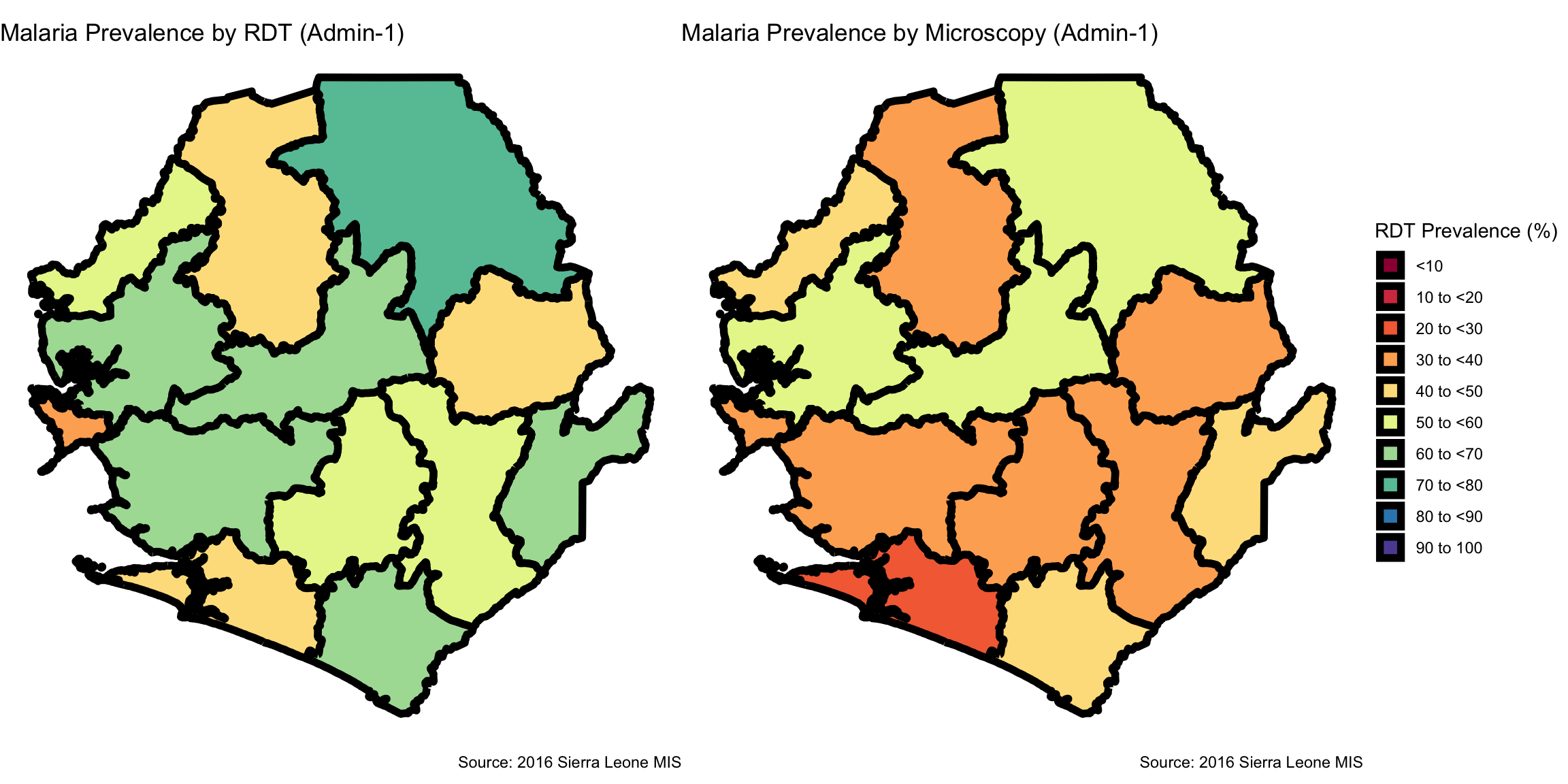
### Step 2: Visualize Subnational Indicator Data -------------------------------
# categorize prevalence percentages
prev_final <- prev_final |>
  dplyr::mutate(
    prev_cat = cut(
      pct,
      breaks = c(0, 10, 20, 30, 40, 50, 60, 70, 80, 90, 100),
      labels = c(
        "<10",
        "10 to <20",
        "20 to <30",
        "30 to <40",
        "40 to <50",
        "50 to <60",
        "60 to <70",
        "70 to <80",
        "80 to <90",
        "90 to 100"
      ),
      include.lowest = TRUE,
      right = FALSE
    )
  )

# visualize RDT-based prevalence
map_rdt <- prev_final |>
  dplyr::filter(indicator == "Malaria prevalence (RDT)") |>
  ggplot2::ggplot() +
  ggplot2::geom_sf(
    ggplot2::aes(fill = prev_cat),
    color = "black",
    size = 2,
    show.legend = TRUE
  ) +
  ggplot2::scale_fill_manual(
    name = "RDT Prevalence (%)",
    values = c(
      "<10" = "#9E0142",
      "10 to <20" = "#D53E4F",
      "20 to <30" = "#F46D43",
      "30 to <40" = "#FDAE61",
      "40 to <50" = "#FEE08B",
      "50 to <60" = "#E6F598",
      "60 to <70" = "#ABDDA4",
      "70 to <80" = "#66C2A5",
      "80 to <90" = "#3288BD",
      "90 to 100" = "#5E4FA2"
    ),
    drop = FALSE
  ) +
  ggplot2::labs(
    title = "Malaria Prevalence by RDT (Admin-1)",
    caption = "Source: 2016 Sierra Leone MIS"
  ) +
  ggplot2::theme_void()

# microscopy map
map_mic <- prev_final |>
  dplyr::filter(indicator != "Malaria prevalence (RDT)") |>
  ggplot2::ggplot() +
  ggplot2::geom_sf(
    ggplot2::aes(fill = prev_cat),
    color = "black",
    size = 2,
    show.legend = TRUE
  ) +
  ggplot2::scale_fill_manual(
    name = "Microscopy Prevalence (%)",
    values = c(
      "<10" = "#9E0142",
      "10 to <20" = "#D53E4F",
      "20 to <30" = "#F46D43",
      "30 to <40" = "#FDAE61",
      "40 to <50" = "#FEE08B",
      "50 to <60" = "#E6F598",
      "60 to <70" = "#ABDDA4",
      "70 to <80" = "#66C2A5",
      "80 to <90" = "#3288BD",
      "90 to 100" = "#5E4FA2"
    ),
    drop = FALSE
  ) +
  ggplot2::labs(
    title = "Malaria Prevalence by Microscopy (Admin-1)",
    caption = "Source: 2016 Sierra Leone MIS"
  ) +
  ggplot2::theme_void()

# display maps side-by-side with shared legend
cowplot::plot_grid(
  map_rdt + ggplot2::theme(legend.position = "none"),
  map_mic + ggplot2::theme(legend.position = "none"),
  cowplot::get_legend(map_rdt),
  ncol = 3,
  rel_widths = c(1, 1, 0.3)
)
# save RDT map
ggplot2::ggsave(
  plot = map_rdt,
  filename = here::here(
    "03_output/3a_figures/malaria_prev_rdt_adm2.png"
  ),
  width = 12,
  height = 9,
  dpi = 300
)

# save microscopy map
ggplot2::ggsave(
  plot = map_mic,
  filename = here::here(
    "03_output/3a_figures/malaria_prev_mic_adm2.png"
  ),
  width = 12,
  height = 9,
  dpi = 300
)
### Step 3: Save Processed Malaria Prevalence Indicators -----------------------
# define save directory
save_path <- here::here("1.6_health_systems/1.6a_dhs")

# save final joined malaria prevalence data
rio::export(
  prev_final |> sf::st_drop_geometry(),
  here::here(
    save_path, "processed", "final_malaria_prev_sle_adm2.csv"
  )
)

# save final joined malaria prevalence data
rio::export(
  prev_final,
  here::here(
    save_path, "processed", "final_malaria_prev_sle_adm2.rds"
  )
)