Reporting rates • sntutils

Before any stratification, trend analysis or modelling step, an SNT analyst needs to know how completely facilities are reporting. calculate_reporting_metrics() is the workhorse: it answers the “who reported, when, where” question in three different shapes.

For the related question - are the values they reported internally consistent and free of outliers - see the Data quality article.

We use the Sierra Leone DHIS2 sample shipped with the package throughout.

library(sntutils)

sl_dhis2 <- read(
  system.file("extdata", "sl_exmaple_dhis2.rds", package = "sntutils")
) |>
  dplyr::rename(year_mon = date) |>
  dplyr::filter(year_mon >= "2020.01") |>
  dplyr::mutate(
    hf_uid    = vdigest(paste0(adm1, adm2, hf), algo = "xxhash32"),
    record_id = vdigest(paste(hf_uid, year_mon),  algo = "xxhash32")
  )

For the methodology and conceptual background behind the steps in this article, please check the SNT Code Library:

Reporting rates - what reporting rate measures and how to interpret it.
Active facility status - the denominator logic in plain English.

What “reporting rate” actually means here

calculate_reporting_metrics() computes the completeness of routine reporting by checking whether health facilities have submitted valid data for a specified set of indicators over time. It calculates rates for one or more target variables (vars_of_interest) against an expectation set defined by the key indicators (key_indicators).

A facility counts as reporting in a given year-month if any of the selected vars_of_interest is non-missing. A facility is included in the denominator for a given year-month only if it has already reported on any of the key_indicators at or before that month. This prevents newly-opened facilities from dragging the historic non-reporting rate down.

Let:

$a$ - administrative unit (e.g. district)
$t$ - time period (year-month)
$f$ - facility in $a$
key_indicators - variables used to determine whether a facility is active, e.g. "test", "treat", "conf", "pres", "allout"
vars_of_interest - variables we want the reporting rate for, e.g. "conf", "pres"

The reporting rate for unit $a$ in period $t$ is

$\text{Reporting Rate}_{a,t} \;=\; \frac{o_{a,t}}{e_{a,t}}$

where

$o_{a,t}$ - facilities in $a$ that reported any value in vars_of_interest during $t$
$e_{a,t}$ - facilities in $a$ whose first-ever report on any key_indicators occurred on or before $t$ .

Worked example

Suppose we want the reporting rate for district $d$ in March:

6 facilities in $d$
all 6 have first-reported on at least one key indicator on or before March
4 of them reported on "conf" in March

$\text{Reporting Rate}_{d,\text{Mar}} \;=\; \frac{4}{6} \;=\; 0.667$

Scenario 1 - Facility-level reporting / missing rate

This is the rate you almost always want when reporting to a country team. It uses an evolving denominator (facilities that have ever reported) so the early months of a new system aren’t punished.

calculate_reporting_metrics(
  data             = sl_dhis2,
  vars_of_interest = c("conf", "pres"),
  x_var            = "year_mon",
  y_var            = "adm2",
  hf_col           = "hf_uid",
  key_indicators   = c("allout", "test", "treat", "conf", "pres")
) |>
  utils::tail()
#> # A tibble: 6 × 6
#>   year_mon adm2                                  rep   exp reprate missrate
#>   <chr>    <chr>                               <int> <int>   <dbl>    <dbl>
#> 1 2023-12  Moyamba District Council              106   108   0.981   0.0185
#> 2 2023-12  Port Loko City Council                  2     2   1       0
#> 3 2023-12  Port Loko District Council             99   103   0.961   0.0388
#> 4 2023-12  Pujehun District Council               96   104   0.923   0.0769
#> 5 2023-12  Tonkolili District Council            109   115   0.948   0.0522
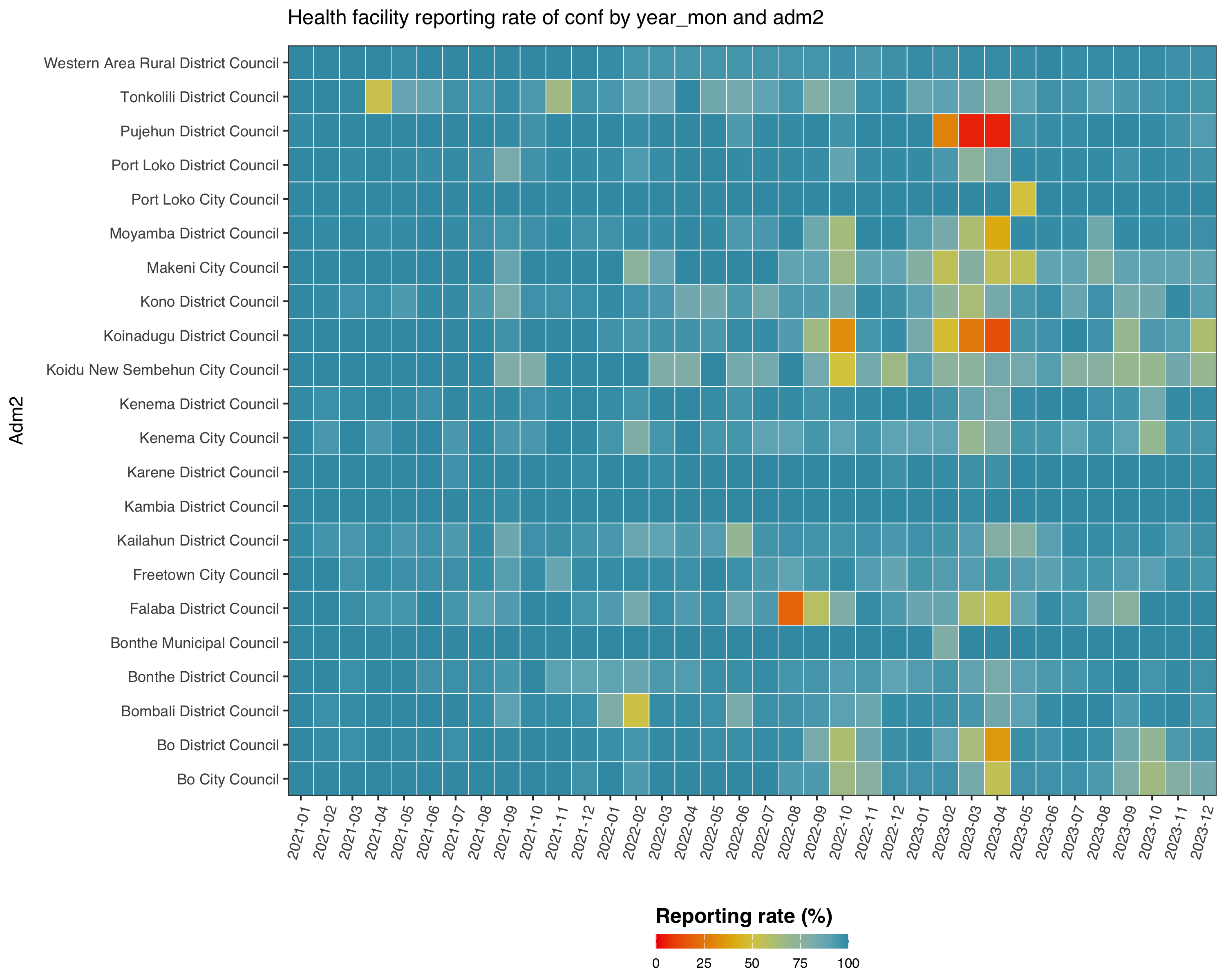
#> 6 2023-12  Western Area Rural District Council    62    64   0.969   0.0312

The plot version is reporting_rate_plot() with the same arguments:

reporting_rate_plot(
  data             = sl_dhis2,
  vars_of_interest = "conf",
  x_var            = "year_mon",
  y_var            = "adm2",
  hf_col           = "hf_uid",
  key_indicators   = c("allout", "test", "treat", "conf", "pres")
)

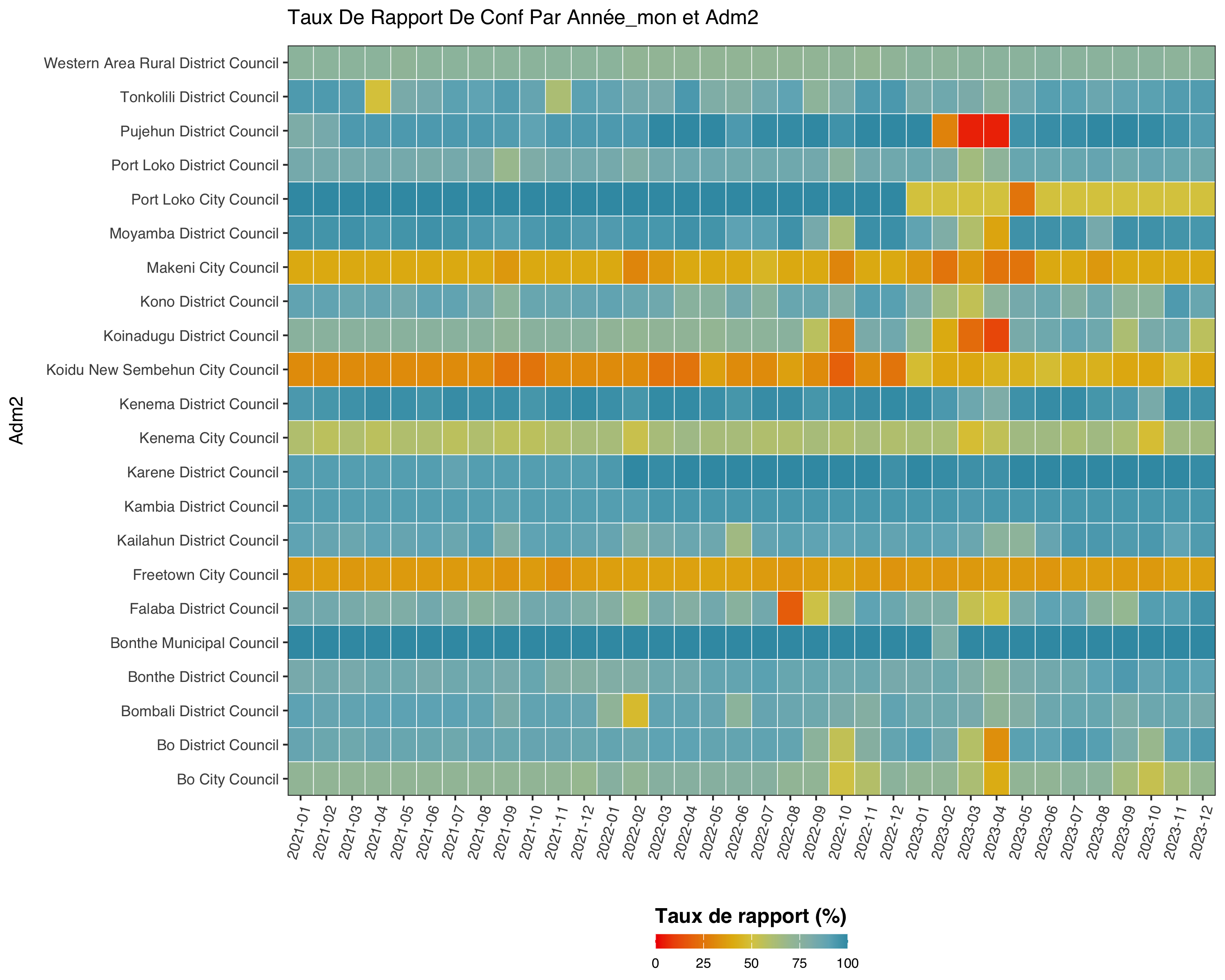
Scenario 2 - Reporting rate by two dimensions

When we want a heatmap of completeness across time × space for one or more variables, without the activity-based denominator, drop hf_col and key_indicators:

calculate_reporting_metrics(
  data             = sl_dhis2,
  vars_of_interest = c("conf", "pres"),
  x_var            = "year_mon",
  y_var            = "adm2"
) |>
  utils::head()
#> # A tibble: 6 × 7
#>   year_mon adm2                     variable   exp   rep reprate missrate
#>   <chr>    <chr>                    <chr>    <int> <int>   <dbl>    <dbl>
#> 1 2021-01  Bo City Council          conf        39    28   0.718   0.282
#> 2 2021-01  Bo City Council          pres        39    28   0.718   0.282
#> 3 2021-01  Bo District Council      conf       129   113   0.876   0.124
#> 4 2021-01  Bo District Council      pres       129   113   0.876   0.124
#> 5 2021-01  Bombali District Council conf        81    73   0.901   0.0988
#> 6 2021-01  Bombali District Council pres        81    73   0.901   0.0988

And the matching plot, this time with French labels:

reporting_rate_plot(
  data             = sl_dhis2,
  vars_of_interest = "conf",
  x_var            = "year_mon",
  y_var            = "adm2",
  target_language  = "fr"
)

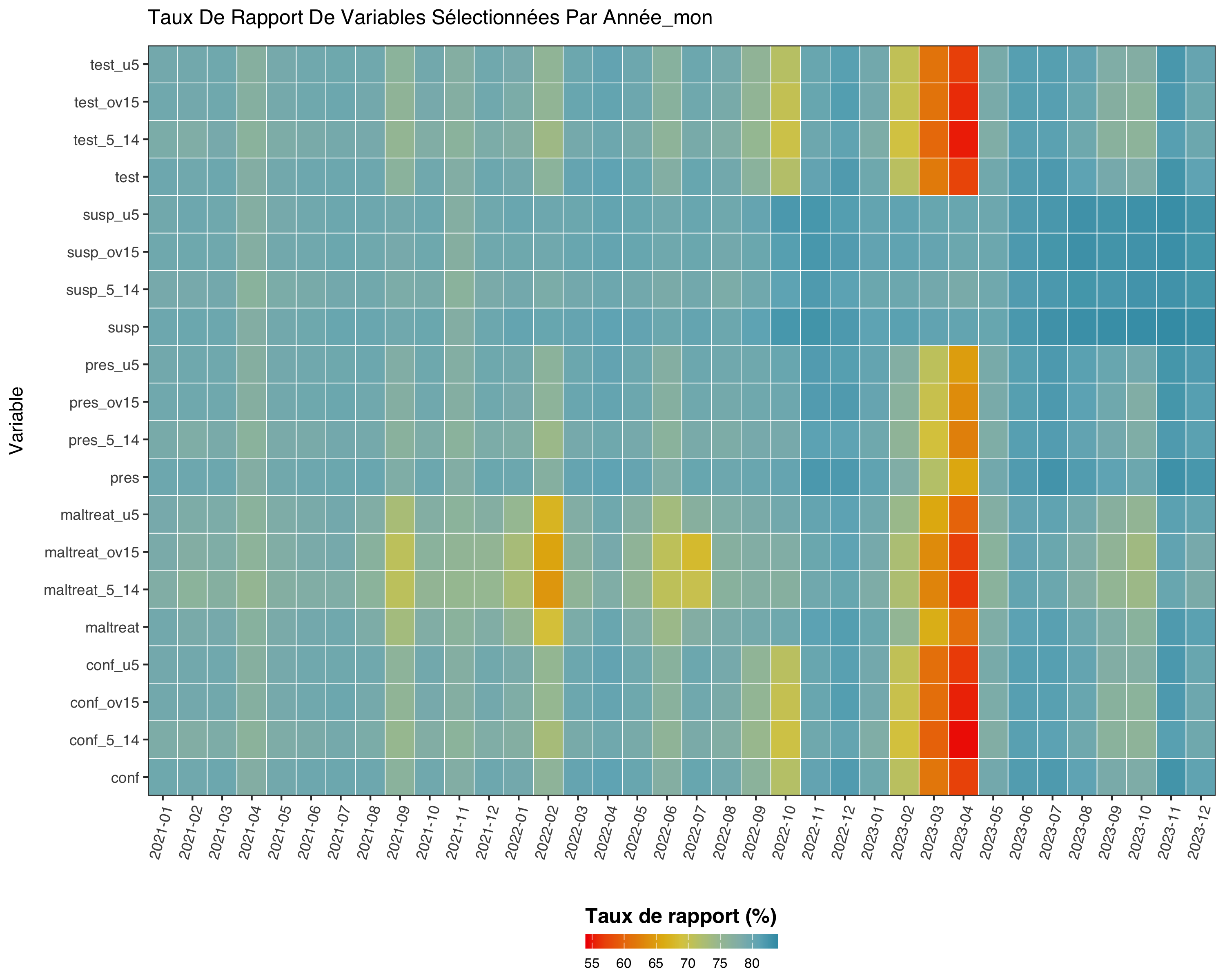
Scenario 3 - Reporting rates over time

To see when each variable starts being reported (and where it stops), drop y_var entirely:

vars <- c(
  "test", "test_u5", "test_5_14", "test_ov15",
  "susp", "susp_u5", "susp_5_14", "susp_ov15",
  "pres", "pres_u5", "pres_5_14", "pres_ov15",
  "conf", "conf_u5", "conf_5_14", "conf_ov15",
  "maltreat", "maltreat_u5", "maltreat_5_14", "maltreat_ov15"
)

reporting_rate_plot(
  sl_dhis2,
  full_range       = FALSE,
  vars_of_interest = vars,
  x_var            = "year_mon",
  target_language  = "fr"
)

Date-based reporting

calculate_reporting_metrics_dates() is the variant for facility registries that record opening and closing dates rather than month-by-month reporting. It computes the share of facilities active in each period from start_col / end_col columns.

Mapping reporting rates

reporting_rate_map() joins the metrics tibble to an admin shapefile and renders a small-multiples map. It accepts everything calculate_reporting_metrics() does, plus an sf argument:

reporting_rate_map(
  data            = sl_dhis2,
  shapefile       = sle_adm2_clean,
  adm_var         = "adm2",
  vars_of_interest = "conf",
  x_var           = "year",
  hf_col          = "hf_uid",
  key_indicators  = c("allout", "test", "treat", "conf", "pres"),
  target_language = "en"
)

Facility activity classification

For deeper diagnostics, classify_facility_activity() labels each facility-month as active, inactive, never-reported or discontinued, using a configurable rolling window. facility_reporting_plot() then renders a tiled timeline so we can spot facilities that stopped reporting in mid-2022 or never came online:

hf_status <- classify_facility_activity(
  data             = sl_dhis2,
  hf_col           = "hf_uid",
  x_var            = "year_mon",
  vars_of_interest = c("conf", "pres", "test"),
  nonreport_window = 6
)

facility_reporting_plot(
  hf_status,
  facet_by = "adm2"
)

get_active_facilities() returns just the active subset, ready to feed back into a filtered analysis.

compare_methods_plot() lets us compare two reporting-rule choices (e.g. any indicator vs all indicators) on the same data.

validate_routine_hf_data() is the upstream sanity check - it runs a battery of structural checks on a routine HF dataset (required columns, parseable dates, plausible value ranges) before any of the reporting-rate functions get to it. Run it once at ingest.

A reporting-rate pipeline, end to end

# 1. structural validation
validate_routine_hf_data(
  data       = sl_dhis2,
  hf_col     = "hf_uid",
  date_col   = "year_mon",
  vars       = c("conf", "pres", "test")
)

# 2. district-month reporting rates for the variables we'll model on
rates <- calculate_reporting_metrics(
  data             = sl_dhis2,
  vars_of_interest = c("conf", "pres"),
  x_var            = "year_mon",
  y_var            = "adm2",
  hf_col           = "hf_uid",
  key_indicators   = c("allout", "test", "treat", "conf", "pres")
)

# 3. facility-level activity so we can mask non-reporting facilities later
activity <- classify_facility_activity(
  data             = sl_dhis2,
  hf_col           = "hf_uid",
  x_var            = "year_mon",
  vars_of_interest = c("conf", "pres", "test"),
  nonreport_window = 6
)

# 4. map of completeness in French, ready for the country-team report
reporting_rate_map(
  data            = sl_dhis2,
  shapefile       = sle_adm2_clean,
  adm_var         = "adm2",
  vars_of_interest = "conf",
  x_var           = "year",
  hf_col          = "hf_uid",
  key_indicators  = c("allout", "test", "treat", "conf", "pres"),
  target_language = "fr"
)

rates and activity are the inputs the Data quality article picks up from here.