Data quality • sntutils

Reporting completeness (covered in Reporting rates) tells us whether facilities reported. This article covers the next two quality questions: are the values they reported internally consistent, and are there outliers that need correcting before modelling?

library(sntutils)

sl_dhis2 <- read(
  system.file("extdata", "sl_exmaple_dhis2.rds", package = "sntutils")
) |>
  dplyr::rename(year_mon = date) |>
  dplyr::filter(year_mon >= "2020.01") |>
  dplyr::mutate(
    hf_uid    = vdigest(paste0(adm1, adm2, hf), algo = "xxhash32"),
    record_id = vdigest(paste(hf_uid, year_mon),  algo = "xxhash32")
  )

For the methodology and conceptual background behind the steps in this article, please check the SNT Code Library:

Quality control (consistency checks) - cascade logic and red flags.
Outlier detection - when to use mean, median or IQR rules.
Outlier correction - decision rules for replacing flagged values.
Missing data - patterns and what to do about them.
Imputation - replacement strategies in context.

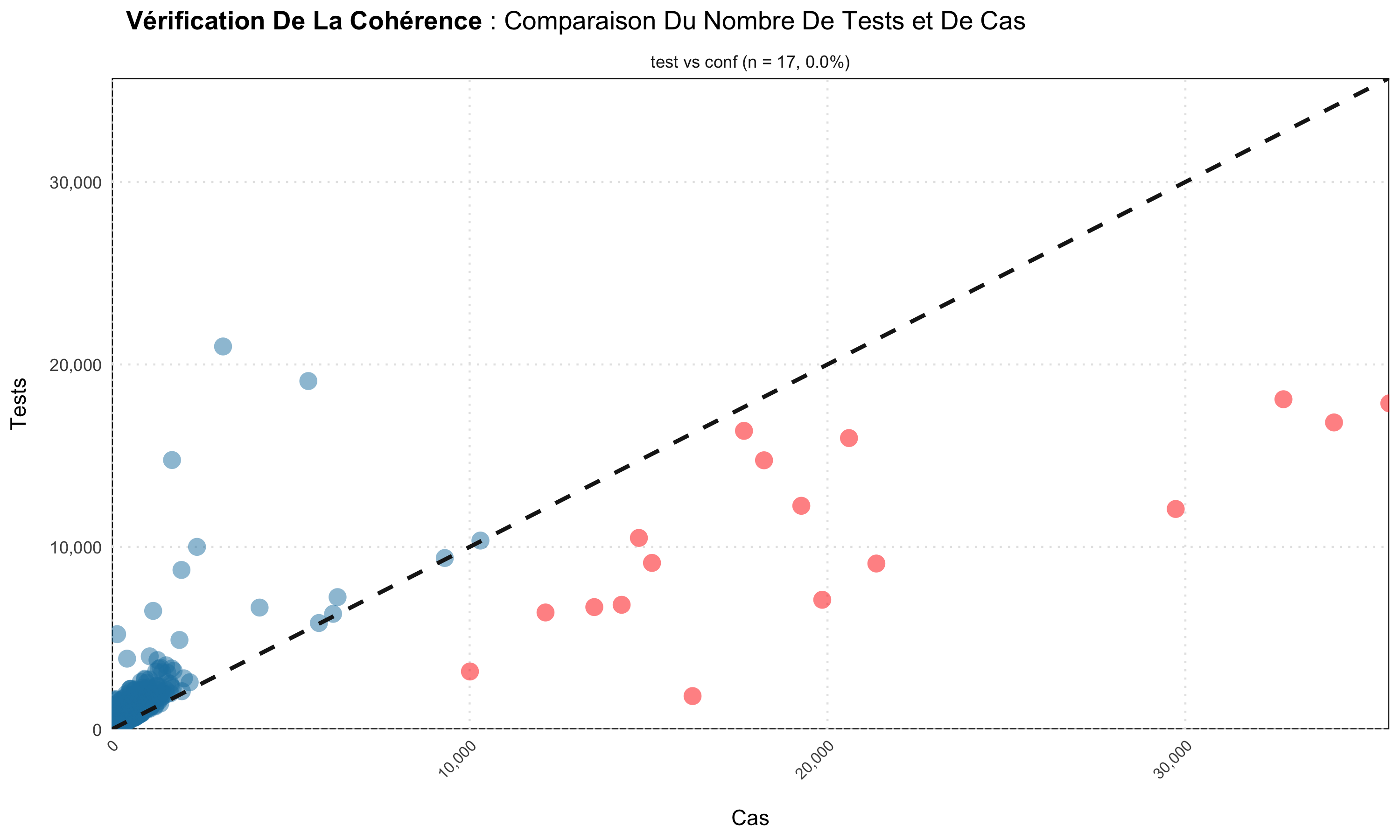
Consistency checks

The malaria care cascade has a fixed direction: outpatients ≥ suspected ≥ tested ≥ confirmed ≥ treated, and admissions ≥ malaria admissions ≥ malaria deaths. consistency_check() flags facility-months that violate any of these and renders a scatter of input vs output with the violating points highlighted.

Common cascade checks include:

All outpatients ≥ suspected malaria
Malaria tests ≥ confirmed cases
Confirmed cases ≥ cases treated
All admissions ≥ malaria admissions
Malaria admissions ≥ malaria deaths

# tests (inputs) vs confirmed cases (outputs)
consistency_check(
  sl_dhis2,
  inputs  = c("test"),
  outputs = c("conf")
)

# save the plot
consistency_check(
  sl_dhis2,
  inputs    = c("test"),
  outputs   = c("conf"),
  save_plot = TRUE,
  plot_path = "plots/consistency_check_plots"
)

# translated labels (French)
consistency_check(
  sl_dhis2,
  inputs          = c("test"),
  outputs         = c("conf"),
  target_language = "fr"
)

# multiple cascades at once
consistency_check(
  sl_dhis2,
  inputs          = c("test", "conf", "alladm"),
  outputs         = c("conf", "maltreat", "maladm"),
  target_language = "fr"
)

Mapping consistency

consistency_map() renders a choropleth of cascade-violation rates by admin unit - useful for spotting whether the cascade is breaking in particular districts vs. system-wide:

consistency_map(
  data       = sl_dhis2,
  shapefile  = sle_adm2_clean,
  input_var  = "test",
  output_var = "conf",
  adm_var    = "adm2",
  x_var      = "year",
  language   = "en"
)

Outlier detection

detect_outliers() flags unusual values in a numeric column using three complementary methods, with detection done within groups of admin unit × facility × year so seasonal and contextual variation isn’t mistaken for noise:

Mean ± 3 SD - classic, parametric, sensitive to extremes.
Median ± 15 × MAD - robust, the workhorse for surveillance data.
Tukey’s fences - quartile-based, tunable via iqr_multiplier.

outlier_results <- detect_outliers(
  data       = sl_dhis2,
  column     = "conf",
  yearmon    = "year_mon",
  record_id  = "record_id",
  adm1       = "adm1",
  adm2       = "adm2",
  iqr_multiplier = 2
)

outlier_results |>
  dplyr::select(record_id, value, outliers_iqr, outliers_median, outliers_mean) |>
  utils::tail()
#> # A tibble: 6 × 5
#>   record_id value outliers_iqr outliers_median outliers_mean
#>   <chr>     <dbl> <chr>        <chr>           <chr>
#> 1 e8947016    321 normal value normal value    normal value
#> 2 28b6ea90    353 normal value normal value    normal value
#> 3 8aa281d9    246 normal value normal value    normal value
#> 4 8b337b53    305 normal value normal value    normal value
#> 5 7358f600    284 normal value normal value    normal value
#> 6 499f0390    309 normal value normal value    normal value

The output has one row per record. Join back on record_id and filter or correct as needed.

Visualising outliers

outlier_plot() returns a list of ggplot objects - one per method - faceted by district and coloured by status. Facet labels show the share of outliers in each district.

plots <- outlier_plot(
  data      = sl_dhis2,
  column    = "conf",
  record_id = "record_id",
  adm1      = "adm1",
  adm2      = "adm2",
  yearmon   = "year_mon",
  methods   = c("iqr", "median", "mean")
)

plots$iqr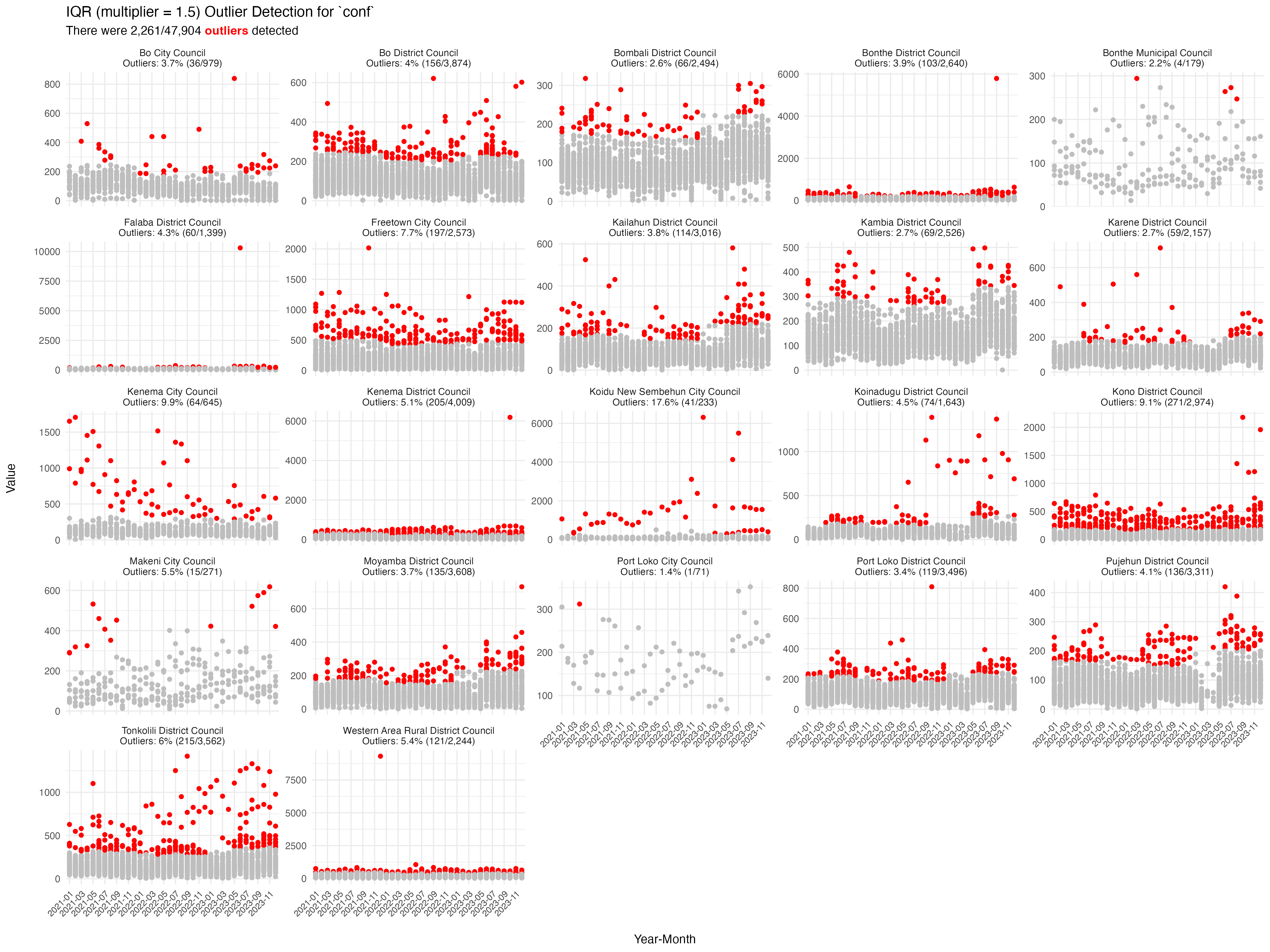

plots$median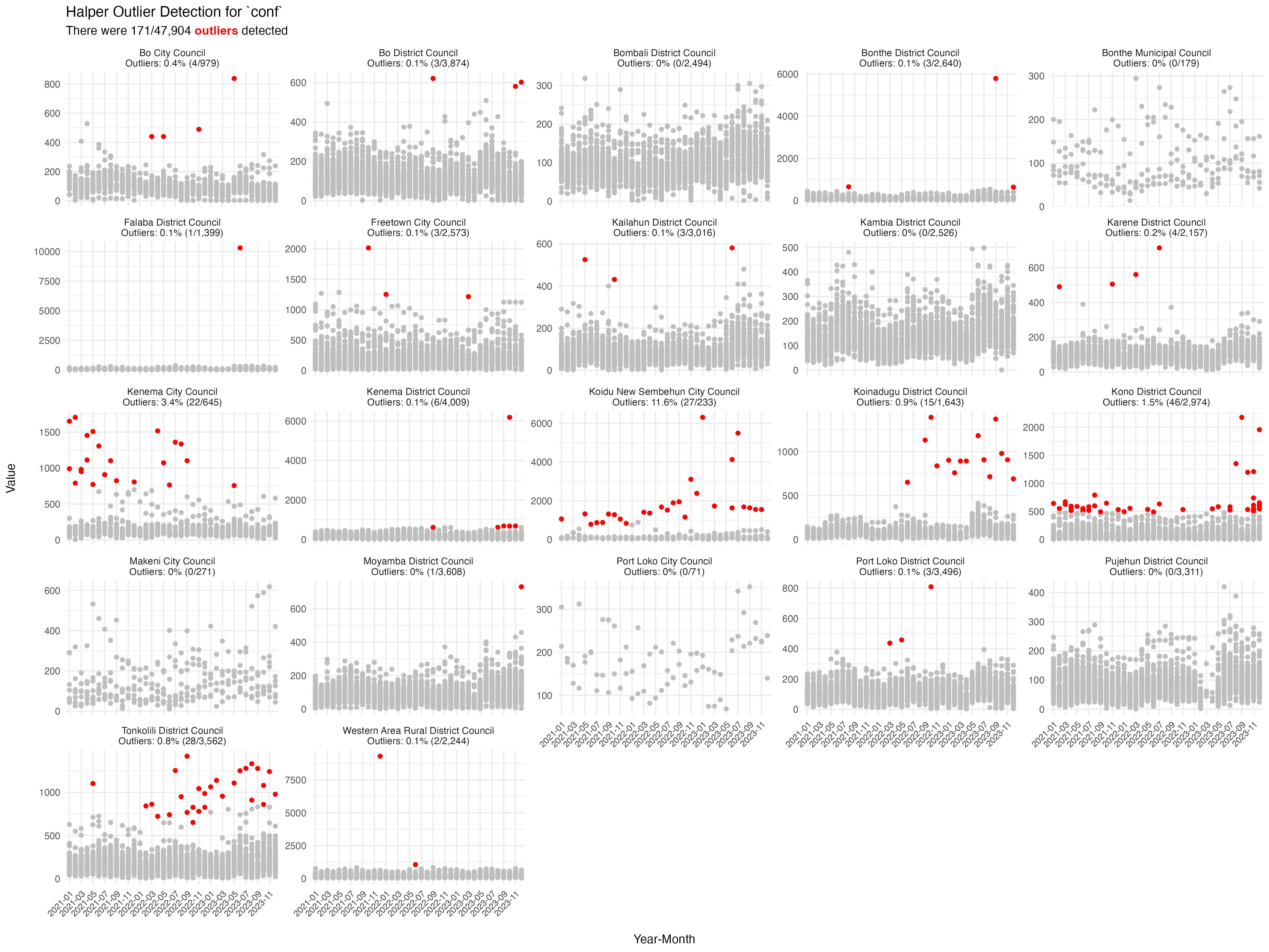

plots$mean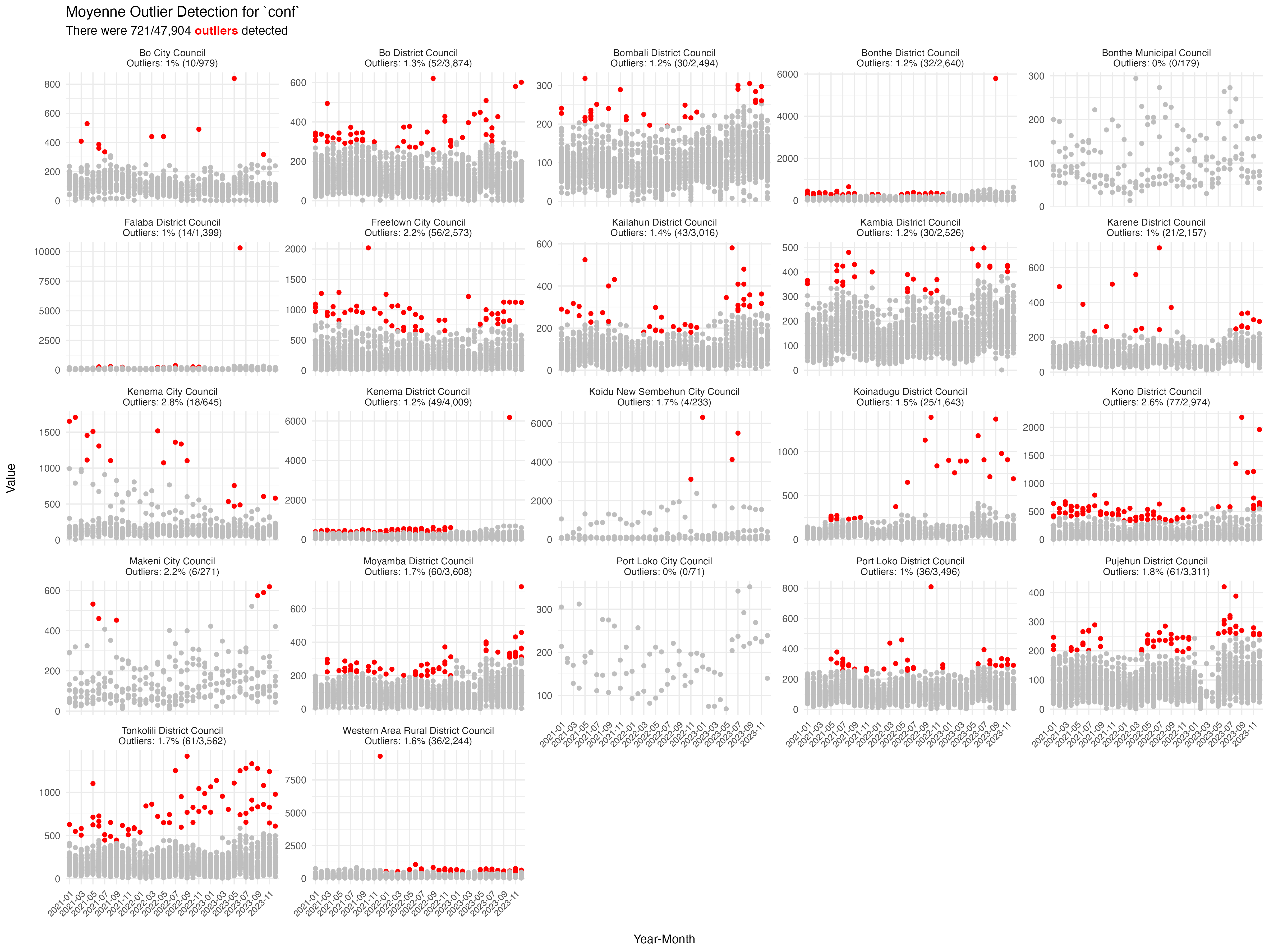

Correcting outliers and imputing missingness

Once outliers are identified, correct_outliers() replaces flagged values using one of several strategies:

sl_corrected <- correct_outliers(
  data        = sl_dhis2,
  outliers    = outlier_results,
  column      = "conf",
  method      = "moving_average",
  flag_method = "iqr"
)

The supporting functions:

impute_outlier_ma() - moving-average imputation; the workhorse inside correct_outliers() when method = "moving_average".
impute_higher_admin() - borrow strength from the parent admin unit when the facility’s own history is too sparse to support a within-unit estimate.
fallback_diff(), fallback_row_sum(), safe_sum() - defensive numerical helpers used inside the imputation paths. They tolerate all-NA rows, return zeros where appropriate, and refuse to silently sum characters.

A quality pipeline, end to end

# 1. cascade consistency at the facility-month level
cascade <- consistency_check(
  data      = sl_dhis2,
  inputs    = c("test", "conf"),
  outputs   = c("conf", "maltreat"),
  show_plot = FALSE
)

# 2. detect outliers on confirmed cases
outliers <- detect_outliers(
  data      = sl_dhis2,
  column    = "conf",
  yearmon   = "year_mon",
  record_id = "record_id",
  adm1      = "adm1",
  adm2      = "adm2"
)

# 3. correct using a moving average, flagged by the robust median rule
sl_clean <- correct_outliers(
  data        = sl_dhis2,
  outliers    = outliers,
  column      = "conf",
  method      = "moving_average",
  flag_method = "median"
)

The output is sl_clean - same shape as the input but with flagged-and-replaced values - plus diagnostic objects (cascade, outliers) you can hand to reviewers as evidence for why each record was edited.